Section 2.3The Limit Laws
In the previous section, we evaluated limits by looking at graphs or by constructing a table of values. In this section, we establish laws for calculating limits and learn how to apply these laws. In the Student Project at the end of this section, you have the opportunity to apply these limit laws to derive the formula for the area of a circle by adapting a method devised by the Greek mathematician Archimedes. We begin by restating two useful limit results from the previous section. These two results, together with the limit laws, serve as a foundation for calculating many limits.
Evaluating Limits with the Limit Laws
The first two limit laws were stated in the previous section and we repeat them here. These basic results, together with the other limit laws, allow us to evaluate limits of many algebraic functions.
For any real number a and any constant c,
\[\underset{x\to a}{\text{lim}}x=a\]
\[\underset{x\to a}{\text{lim}}c=c\]
Evaluate each of the following limits using the basic limit results above.
- \(\underset{x\to 2}{\text{lim}}x\)
- \(\underset{x\to 2}{\text{lim}}5\)
Which limit law from just above applies to each piece — the variable itself, or a constant?
- The limit of x as x approaches a is a: \(\underset{x\to 2}{\text{lim}}x=2.\)
- The limit of a constant is that constant: \(\underset{x\to 2}{\text{lim}}5=5.\)
We now take a look at the limit laws, the individual properties of limits. The proofs that these laws hold are omitted here.
Let \(f(x)\) and \(g(x)\) be defined for all \(x\ne a\) over some open interval containing a. Assume that L and M are real numbers such that \(\underset{x\to a}{\text{lim}}f(x)=L\) and \(\underset{x\to a}{\text{lim}}g(x)=M.\) Let c be a constant. Then, each of the following statements holds:
Sum law for limits: \(\underset{x\to a}{\text{lim}}(f(x)+g(x))=\underset{x\to a}{\text{lim}}f(x)+\underset{x\to a}{\text{lim}}g(x)=L+M\)
Difference law for limits: \(\underset{x\to a}{\text{lim}}(f(x)-g(x))=\underset{x\to a}{\text{lim}}f(x)-\underset{x\to a}{\text{lim}}g(x)=L-M\)
Constant multiple law for limits: \(\underset{x\to a}{\text{lim}}cf(x)=c·\underset{x\to a}{\text{lim}}f(x)=cL\)
Product law for limits: \(\underset{x\to a}{\text{lim}}(f(x)·g(x))=\underset{x\to a}{\text{lim}}f(x)·\underset{x\to a}{\text{lim}}g(x)=L·M\)
Quotient law for limits: \(\underset{x\to a}{\text{lim}}\frac{f(x)}{g(x)}=\frac{\underset{x\to a}{\text{lim}}f(x)}{\underset{x\to a}{\text{lim}}g(x)}=\frac{L}{M}\) for \(M\ne 0\)
Power law for limits: \(\underset{x\to a}{\text{lim}}{(f(x))}^{n}={(\underset{x\to a}{\text{lim}}f(x))}^{n}={L}^{n}\) for every positive integer n.
Root law for limits: \(\underset{x\to a}{\text{lim}}\sqrt[n]{f(x)}=\sqrt[n]{\underset{x\to a}{\text{lim}}f(x)}=\sqrt[n]{L}\) for all L if n is odd and for \(L\ge 0\) if n is even and \(f(x)\ge 0\) .
We now practice applying these limit laws to evaluate a limit.
Use the limit laws to evaluate \(\underset{x\to -3}{\text{lim}}(4x+2).\)
Break the sum into two limits, then pull the constant out front before substituting.
Let’s apply the limit laws one step at a time to be sure we understand how they work. We need to keep in mind the requirement that, at each application of a limit law, the new limits must exist for the limit law to be applied.
\(\begin{array}{lllll}\underset{x\to -3}{\text{lim}}(4x+2) & =\underset{x\to -3}{\text{lim}}4x+\underset{x\to -3}{\text{lim}}2 & & & \text{Apply the sum law.} \\ & =4·\underset{x\to -3}{\text{lim}}x+\underset{x\to -3}{\text{lim}}2 & & & \text{Apply the constant multiple law.} \\ & =4·(-3)+2=-10. & & & \text{Apply the basic limit results and simplify.}\end{array}\)
Use the limit laws to evaluate \(\underset{x\to 2}{\text{lim}}\frac{2{x}^{2}-3x+1}{{x}^{3}+4}.\)
The denominator doesn't vanish at x=2, so which law lets you split numerator and denominator?
To find this limit, we need to apply the limit laws several times. Again, we need to keep in mind that as we rewrite the limit in terms of other limits, each new limit must exist for the limit law to be applied.
\(\begin{array}{lllll} \\ \\ \underset{x\to 2}{\text{lim}}\frac{2{x}^{2}-3x+1}{{x}^{3}+4} & =\frac{\underset{x\to 2}{\text{lim}}(2{x}^{2}-3x+1)}{\underset{x\to 2}{\text{lim}}({x}^{3}+4)} & & & \text{Apply the quotient law, making sure that.}\,{(2)}^{3}+4\ne 0 \\ & =\frac{2·\underset{x\to 2}{\text{lim}}{x}^{2}-3·\underset{x\to 2}{\text{lim}}x+\underset{x\to 2}{\text{lim}}1}{\underset{x\to 2}{\text{lim}}{x}^{3}+\underset{x\to 2}{\text{lim}}4} & & & \text{Apply the sum law and constant multiple law.} \\ & =\frac{2·{(\underset{x\to 2}{\text{lim}}x)}^{2}-3·\underset{x\to 2}{\text{lim}}x+\underset{x\to 2}{\text{lim}}1}{{(\underset{x\to 2}{\text{lim}}x)}^{3}+\underset{x\to 2}{\text{lim}}4} & & & \text{Apply the power law.} \\ & =\frac{2(4)-3(2)+1}{{(2)}^{3}+4}=\frac{1}{4}. & & & \text{Apply the basic limit laws and simplify.}\end{array}\)
Use the limit laws to evaluate \(\underset{x\to 6}{\text{lim}}(2x-1)\sqrt{x+4}.\) In each step, indicate the limit law applied.
\(11\sqrt{10}\)
Limits of Polynomial and Rational Functions
By now you have probably noticed that, in each of the previous examples, it has been the case that \(\underset{x\to a}{\text{lim}}f(x)=f(a).\) This is not always true, but it does hold for all polynomials for any choice of a and for all rational functions at all values of a for which the rational function is defined.
Let \(p(x)\) and \(q(x)\) be polynomial functions. Let a be a real number. Then,
\[\underset{x\to a}{\text{lim}}p(x)=p(a)\]
\[\underset{x\to a}{\text{lim}}\frac{p(x)}{q(x)}=\frac{p(a)}{q(a)}\,\text{when}\,q(a)\ne 0.\]
To see that this theorem holds, consider the polynomial \(p(x)={c}_{n}{x}^{n}+{c}_{n-1}{x}^{n-1}+⋯+{c}_{1}x+{c}_{0}.\) By applying the sum, constant multiple, and power laws, we end up with
\[\begin{array}{ll}\underset{x\to a}{\text{lim}}p(x) & =\underset{x\to a}{\text{lim}}({c}_{n}{x}^{n}+{c}_{n-1}{x}^{n-1}+⋯+{c}_{1}x+{c}_{0}) \\ & ={c}_{n}{(\underset{x\to a}{\text{lim}}x)}^{n}+{c}_{n-1}{(\underset{x\to a}{\text{lim}}x)}^{n-1}+⋯+{c}_{1}(\underset{x\to a}{\text{lim}}x)+\underset{x\to a}{\text{lim}}{c}_{0} \\ & ={c}_{n}{a}^{n}+{c}_{n-1}{a}^{n-1}+⋯+{c}_{1}a+{c}_{0} \\ & =p(a).\end{array}\]
It now follows from the quotient law that if \(p(x)\) and \(q(x)\) are polynomials for which \(q(a)\ne 0,\) then
\[\underset{x\to a}{\text{lim}}\frac{p(x)}{q(x)}=\frac{p(a)}{q(a)}.\]
Example 4 applies this result.
Evaluate the \(\underset{x\to 3}{\text{lim}}\frac{2{x}^{2}-3x+1}{5x+4}.\)
Check whether the denominator is zero at x=3 before you decide you can just substitute.
Since 3 is in the domain of the rational function \(f(x)=\frac{2{x}^{2}-3x+1}{5x+4},\) we can calculate the limit by substituting 3 for x into the function. Thus,
\[\underset{x\to 3}{\text{lim}}\frac{2{x}^{2}-3x+1}{5x+4}=\frac{10}{19}.\]
Evaluate \(\underset{x\to -2}{\text{lim}}(3{x}^{3}-2x+7).\)
−13;
Additional Limit Evaluation Techniques
As we have seen, we may evaluate easily the limits of polynomials and limits of some (but not all) rational functions by direct substitution. However, as we saw in the introductory section on limits, it is certainly possible for \(\underset{x\to a}{\text{lim}}f(x)\) to exist when \(f(a)\) is undefined. The following observation allows us to evaluate many limits of this type:
If for all \(x\ne a,f(x)=g(x)\) over some open interval containing a, then \(\underset{x\to a}{\text{lim}}f(x)=\underset{x\to a}{\text{lim}}g(x).\)
To understand this idea better, consider the limit \(\underset{x\to 1}{\text{lim}}\frac{{x}^{2}-1}{x-1}.\)
The function
\[\begin{array}{ll}f(x) & =\frac{{x}^{2}-1}{x-1} \\ & =\frac{(x-1)(x+1)}{x-1}\end{array}\]
and the function \(g(x)=x+1\) are identical for all values of \(x\ne 1.\) The graphs of these two functions are shown in Figure 1.
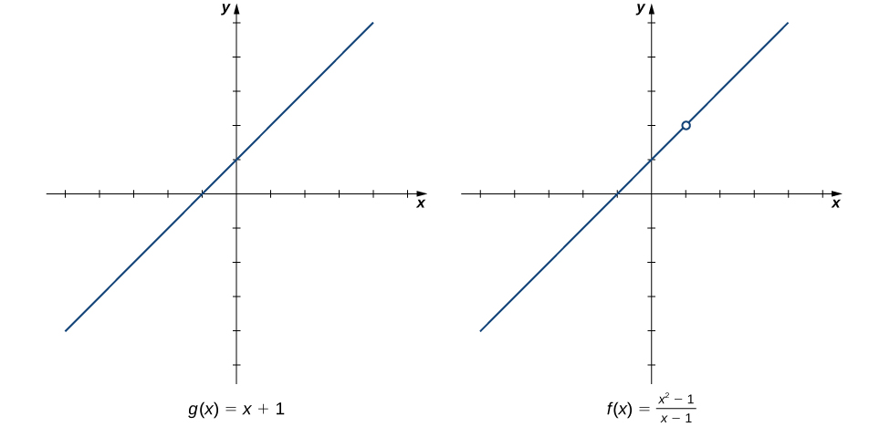
We see that
\[\begin{array}{ll}\underset{x\to 1}{\text{lim}}\frac{{x}^{2}-1}{x-1} & =\underset{x\to 1}{\text{lim}}\frac{(x-1)(x+1)}{x-1} \\ & =\underset{x\to 1}{\text{lim}}(x+1) \\ & =2.\end{array}\]
The limit has the form \(\underset{x\to a}{\text{lim}}\frac{f(x)}{g(x)},\) where \(\underset{x\to a}{\text{lim}}f(x)=0\) and \(\underset{x\to a}{\text{lim}}g(x)=0.\) (In this case, we say that \(f(x)\text{/}g(x)\) has the indeterminate form \(0\text{/}0\text{.)}\) The following Problem-Solving Strategy provides a general outline for evaluating limits of this type.
- First, we need to make sure that our function has the appropriate form and cannot be evaluated immediately using the limit laws.
- We then need to find a function that is equal to \(h(x)=f(x)\text{/}g(x)\) for all \(x\ne a\) over some interval containing a. To do this, we may need to try one or more of the following steps:
- If \(f(x)\) and \(g(x)\) are polynomials, we should factor each function and cancel out any common factors.
- If the numerator or denominator contains a difference involving a square root, we should try multiplying the numerator and denominator by the conjugate of the expression involving the square root.
- If \(f(x)\text{/}g(x)\) is a complex fraction, we begin by simplifying it.
- Last, we apply the limit laws.
The next examples demonstrate the use of this Problem-Solving Strategy. Example 5 illustrates the factor-and-cancel technique; Example 6 shows multiplying by a conjugate. In Example 7, we look at simplifying a complex fraction.
Evaluate \(\underset{x\to 3}{\text{lim}}\frac{{x}^{2}-3x}{2{x}^{2}-5x-3}.\)
Plug in 3 first — the 0/0 form tells you factoring is the move, not the limit laws directly.
Step 1. The function \(f(x)=\frac{{x}^{2}-3x}{2{x}^{2}-5x-3}\) is undefined for \(x=3.\) In fact, if we substitute 3 into the function we get \(0\text{/}0,\) which is indeterminate. Factoring and canceling is a good strategy:
\[\underset{x\to 3}{\text{lim}}\frac{{x}^{2}-3x}{2{x}^{2}-5x-3}=\underset{x\to 3}{\text{lim}}\frac{x(x-3)}{(x-3)(2x+1)}\]
Step 2. For all \(x\ne 3,\frac{{x}^{2}-3x}{2{x}^{2}-5x-3}=\frac{x}{2x+1}.\) Therefore,
\[\underset{x\to 3}{\text{lim}}\frac{x(x-3)}{(x-3)(2x+1)}=\underset{x\to 3}{\text{lim}}\frac{x}{2x+1}.\]
Step 3. Evaluate using the limit laws:
\[\underset{x\to 3}{\text{lim}}\frac{x}{2x+1}=\frac{3}{7}.\]
Evaluate \(\underset{x\to -3}{\text{lim}}\frac{{x}^{2}+4x+3}{{x}^{2}-9}.\)
\(\frac{1}{3}\)
Evaluate \(\underset{x\to -1}{\text{lim}}\frac{\sqrt{x+2}-1}{x+1}.\)
0/0 again, but no common factor to cancel yet — what do you multiply by to clear the square root?
Step 1. \(\frac{\sqrt{x+2}-1}{x+1}\) has the form \(0\text{/}0\) at −1. Let’s begin by multiplying by \(\sqrt{x+2}+1,\) the conjugate of \(\sqrt{x+2}-1,\) on the numerator and denominator:
\[\underset{x\to -1}{\text{lim}}\frac{\sqrt{x+2}-1}{x+1}=\underset{x\to -1}{\text{lim}}\frac{\sqrt{x+2}-1}{x+1}·\frac{\sqrt{x+2}+1}{\sqrt{x+2}+1}.\]
Step 2. We then multiply out the numerator. We don’t multiply out the denominator because we are hoping that the \((x+1)\) in the denominator cancels out in the end:
\[=\underset{x\to -1}{\text{lim}}\frac{x+1}{(x+1)(\sqrt{x+2}+1)}.\]
Step 3. Then we cancel:
\[=\underset{x\to -1}{\text{lim}}\frac{1}{\sqrt{x+2}+1}.\]
Step 4. Last, we apply the limit laws:
\[\underset{x\to -1}{\text{lim}}\frac{1}{\sqrt{x+2}+1}=\frac{1}{2}.\]
Evaluate \(\underset{x\to 5}{\text{lim}}\frac{\sqrt{x-1}-2}{x-5}.\)
\(\frac{1}{4}\)
Evaluate \(\underset{x\to 1}{\text{lim}}\frac{\frac{1}{x+1}-\frac{1}{2}}{x-1}.\)
Clear the fractions inside the fraction first (multiply by the common denominator) before you look for a common factor.
Step 1. \(\frac{\frac{1}{x+1}-\frac{1}{2}}{x-1}\) has the form \(0\text{/}0\) at 1. We simplify the algebraic fraction by multiplying by \(2(x+1)\text{/}2(x+1):\)
\[\underset{x\to 1}{\text{lim}}\frac{\frac{1}{x+1}-\frac{1}{2}}{x-1}=\underset{x\to 1}{\text{lim}}\frac{\frac{1}{x+1}-\frac{1}{2}}{x-1}·\frac{2(x+1)}{2(x+1)}.\]
Step 2. Next, we multiply through the numerators. Do not multiply the denominators because we want to be able to cancel the factor \((x-1)\text{:}\)
\[=\underset{x\to 1}{\text{lim}}\frac{2-(x+1)}{2(x-1)(x+1)}.\]
Step 3. Then, we simplify the numerator:
\[=\underset{x\to 1}{\text{lim}}\frac{-x+1}{2(x-1)(x+1)}.\]
Step 4. Now we factor out −1 from the numerator:
\[=\underset{x\to 1}{\text{lim}}\frac{-(x-1)}{2(x-1)(x+1)}.\]
Step 5. Then, we cancel the common factors of \((x-1)\text{:}\)
\[=\underset{x\to 1}{\text{lim}}\frac{-1}{2(x+1)}.\]
Step 6. Last, we evaluate using the limit laws:
\[\underset{x\to 1}{\text{lim}}\frac{-1}{2(x+1)}=-\frac{1}{4}.\]
Evaluate \(\underset{x\to -3}{\text{lim}}\frac{\frac{1}{x+2}+1}{x+3}.\)
−1;
Example 8 does not fall neatly into any of the patterns established in the previous examples. However, with a little creativity, we can still use these same techniques.
Evaluate \(\underset{x\to 0}{\text{lim}}(\frac{1}{x}+\frac{5}{x(x-5)}).\)
Neither piece has a limit alone — combine the two fractions into one before evaluating.
Both \(1\text{/}x\) and \(5\text{/}x(x-5)\) fail to have a limit at zero. Since neither of the two functions has a limit at zero, we cannot apply the sum law for limits; we must use a different strategy. In this case, we find the limit by performing addition and then applying one of our previous strategies. Observe that
\[\,\begin{array}{ll}\frac{1}{x}+\frac{5}{x(x-5)} & =\frac{x-5+5}{x(x-5)} \\ & =\frac{x}{x(x-5)}.\end{array}\]
Thus,
\[\begin{array}{ll}\underset{x\to 0}{\text{lim}}(\frac{1}{x}+\frac{5}{x(x-5)}) & =\underset{x\to 0}{\text{lim}}\frac{x}{x(x-5)} \\ & =\underset{x\to 0}{\text{lim}}\frac{1}{x-5} \\ & =-\frac{1}{5}.\end{array}\]
Evaluate \(\underset{x\to 3}{\text{lim}}(\frac{1}{x-3}-\frac{4}{{x}^{2}-2x-3}).\)
\(\frac{1}{4}\)
Let’s now revisit one-sided limits. Simple modifications in the limit laws allow us to apply them to one-sided limits. For example, to apply the limit laws to a limit of the form \(\underset{x\to {a}^{-}}{\text{lim}}h(x),\) we require the function \(h(x)\) to be defined over an open interval of the form \((b,a);\) for a limit of the form \(\underset{x\to {a}^{+}}{\text{lim}}h(x),\) we require the function \(h(x)\) to be defined over an open interval of the form \((a,c).\) Example 9 illustrates this point.
Evaluate each of the following limits, if possible.
- \(\underset{x\to {3}^{-}}{\text{lim}}\sqrt{x-3}\)
- \(\underset{x\to {3}^{+}}{\text{lim}}\sqrt{x-3}\)
Think about the domain of the square root function near x=3 before applying any limit law.
Figure 2 illustrates the function \(f(x)=\sqrt{x-3}\) and aids in our understanding of these limits.
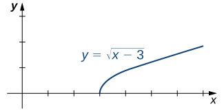
- The function \(f(x)=\sqrt{x-3}\) is defined over the interval \([3,\text{+}\infty ).\) Since this function is not defined to the left of 3, we cannot apply the limit laws to compute \(\underset{x\to {3}^{-}}{\text{lim}}\sqrt{x-3}.\) In fact, since \(f(x)=\sqrt{x-3}\) is undefined to the left of 3, \(\underset{x\to {3}^{-}}{\text{lim}}\sqrt{x-3}\) does not exist.
- Since \(f(x)=\sqrt{x-3}\) is defined to the right of 3, the limit laws do apply to \(\underset{x\to {3}^{+}}{\text{lim}}\sqrt{x-3}.\) By applying these limit laws we obtain \(\underset{x\to {3}^{+}}{\text{lim}}\sqrt{x-3}=0.\)
In Example 10 we look at one-sided limits of a piecewise-defined function and use these limits to draw a conclusion about a two-sided limit of the same function.
For \(f(x)=\left\{\begin{array}{ll}4x-3 & \text{if}\,x<2 \\ {(x-3)}^{2} & \text{if}\,x\ge 2\end{array}\right.,\) evaluate each of the following limits:
- \(\underset{x\to {2}^{-}}{\text{lim}}f(x)\)
- \(\underset{x\to {2}^{+}}{\text{lim}}f(x)\)
- \(\underset{x\to 2}{\text{lim}}f(x)\)
Evaluate the two one-sided limits separately using each formula's own domain, then compare them.
Figure 3 illustrates the function \(f(x)\) and aids in our understanding of these limits.
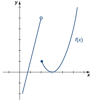
- Since \(f(x)=4x-3\) for all x in \((\text{-}\infty ,2),\) replace \(f(x)\) in the limit with \(4x-3\) and apply the limit laws:
\[\underset{x\to {2}^{-}}{\text{lim}}f(x)=\underset{x\to {2}^{-}}{\text{lim}}(4x-3)=5.\]
- Since \(f(x)={(x-3)}^{2}\) for all x in \((2,\text{+}\infty ),\) replace \(f(x)\) in the limit with \({(x-3)}^{2}\) and apply the limit laws:
\[\underset{x\to {2}^{+}}{\text{lim}}f(x)=\underset{x\to {2}^{+}}{\text{lim}}{(x-3)}^{2}=1.\]
- Since \(\underset{x\to {2}^{-}}{\text{lim}}f(x)=5\) and \(\underset{x\to {2}^{+}}{\text{lim}}f(x)=1,\) we conclude that \(\underset{x\to 2}{\text{lim}}f(x)\) does not exist.
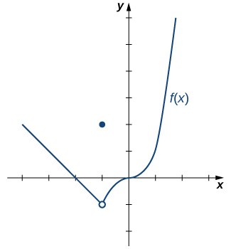
Graph \(f(x)=\left\{\begin{array}{l}-x-2\,\text{if}\,x<\text{-}1 \\ 2\,\text{if}\,x=-1 \\ {x}^{3}\,\text{if}\,x>\text{-}1\end{array}\right.\) and evaluate \(\underset{x\to {-1}^{-}}{\text{lim}}f(x).\)
-1, which crossed the x axis and y axis at the origin.">
\(\underset{x\to {-1}^{-}}{\text{lim}}f(x)=-1\)
We now turn our attention to evaluating a limit of the form \(\underset{x\to a}{\text{lim}}\frac{f(x)}{g(x)},\) where \(\underset{x\to a}{\text{lim}}f(x)=K,\) where \(K\ne 0\) and \(\underset{x\to a}{\text{lim}}g(x)=0.\) That is, \(f(x)\text{/}g(x)\) has the form \(K\text{/}0,K\ne 0\) at a.
Evaluate \(\underset{x\to {2}^{-}}{\text{lim}}\frac{x-3}{{x}^{2}-2x}.\)
Substituting gives −1/0 — factor the denominator and track the sign of each piece as x→2⁻.
Step 1. After substituting in \(x=2,\) we see that this limit has the form \(-1\text{/}0.\) That is, as x approaches 2 from the left, the numerator approaches −1; and the denominator approaches 0. Consequently, the magnitude of \(\frac{x-3}{x(x-2)}\) becomes infinite. To get a better idea of what the limit is, we need to factor the denominator:
\[\underset{x\to {2}^{-}}{\text{lim}}\frac{x-3}{{x}^{2}-2x}=\underset{x\to {2}^{-}}{\text{lim}}\frac{x-3}{x(x-2)}.\]
Step 2. Since \(x-2\) is the only part of the denominator that is zero when 2 is substituted, we then separate \(1\text{/}(x-2)\) from the rest of the function:
\[=\underset{x\to {2}^{-}}{\text{lim}}\frac{x-3}{x}·\frac{1}{x-2}.\]
Step 3. \(\underset{x\to {2}^{-}}{\text{lim}}\frac{x-3}{x}=-\frac{1}{2}\) and \(\underset{x\to {2}^{-}}{\text{lim}}\frac{1}{x-2}=\text{-}\infty .\) Therefore, the product of \((x-3)\text{/}x\) and \(1\text{/}(x-2)\) has a limit of \(\text{+∞:}\)
\[\underset{x\to {2}^{-}}{\text{lim}}\frac{x-3}{{x}^{2}-2x}=\text{+}\infty .\]
Evaluate \(\underset{x\to 1}{\text{lim}}\frac{x+2}{{(x-1)}^{2}}.\)
+∞
The Squeeze Theorem
The techniques we have developed thus far work very well for algebraic functions, but we are still unable to evaluate limits of very basic trigonometric functions. The next theorem, called the squeeze theorem, proves very useful for establishing basic trigonometric limits. This theorem allows us to calculate limits by “squeezing” a function, with a limit at a point a that is unknown, between two functions having a common known limit at a. Figure 4 illustrates this idea.
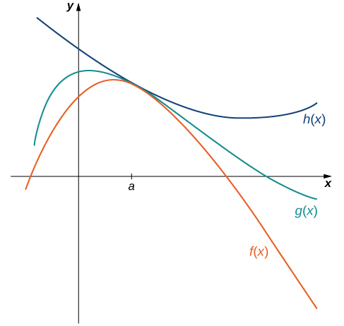
Let \(f(x),g(x),\) and \(h(x)\) be defined for all \(x\ne a\) over an open interval containing a. If
\[f(x)\le g(x)\le h(x)\]
for all \(x\ne a\) in an open interval containing a and
\[\underset{x\to a}{\text{lim}}f(x)=L=\underset{x\to a}{\text{lim}}h(x)\]
where L is a real number, then \(\underset{x\to a}{\text{lim}}g(x)=L.\)
Apply the squeeze theorem to evaluate \(\underset{x\to 0}{\text{lim}}x\,\text{cos}\,x.\)
Squeeze x cos x between two functions you already know the limit of at 0.
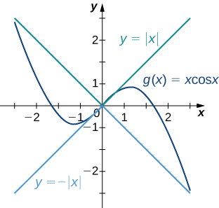
Because \(-1\le \text{cos}\,x\le 1\) for all x, we have \(-\text{|}x\text{|}\le x\,\text{cos}\,x\le \text{|}x\text{|}\) . Since \(\underset{x\to 0}{\text{lim}}(-\text{|}x\text{|})=0=\underset{x\to 0}{\text{lim}}\text{|}x\text{|},\) from the squeeze theorem, we obtain \(\underset{x\to 0}{\text{lim}}x\,\text{cos}\,x=0.\) The graphs of \(f(x)=-\text{|}x\text{|},g(x)=x\,\text{cos}\,x,\) and \(h(x)=\text{|}x\text{|}\) are shown in Figure 5.
Use the squeeze theorem to evaluate \(\underset{x\to 0}{\text{lim}}{x}^{2}\text{sin}\frac{1}{x}.\)
0
We now use the squeeze theorem to tackle several very important limits. Although this discussion is somewhat lengthy, these limits prove invaluable for the development of the material in both the next section and the next chapter. The first of these limits is \(\underset{θ\to 0}{\text{lim}}\text{sin}\,θ.\) Consider the unit circle shown in Figure 6. In the figure, we see that \(\text{sin}\,θ\) is the y-coordinate on the unit circle and it corresponds to the line segment shown in blue. The radian measure of angle θ is the length of the arc it subtends on the unit circle. Therefore, we see that for \(0<θ<\frac{\pi }{2},0<\text{sin}\,θ<θ.\)
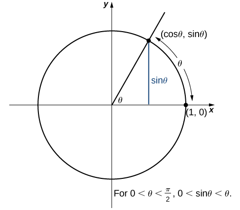
Because \(\underset{θ\to {0}^{+}}{\text{lim}}0=0\) and \(\underset{θ\to {0}^{+}}{\text{lim}}θ=0,\) by using the squeeze theorem we conclude that
\[\underset{θ\to {0}^{+}}{\text{lim}}\text{sin}\,θ=0.\]
To see that \(\underset{θ\to {0}^{-}}{\text{lim}}\text{sin}\,θ=0\) as well, observe that for \(-\frac{\pi }{2}<θ<0,0<\text{-}θ<\frac{\pi }{2}\) and hence, \(0<\text{sin}\,(-θ)<\text{-}θ.\) Consequently, \(0<-\text{sin}\,θ<\text{-}θ.\) It follows that \(0>\text{sin}\,θ>θ.\) An application of the squeeze theorem produces the desired limit. Thus, since \(\underset{θ\to {0}^{+}}{\text{lim}}\text{sin}\,θ=0\) and \(\underset{θ\to {0}^{-}}{\text{lim}}\text{sin}\,θ=0,\)
\[\underset{θ\to 0}{\text{lim}}\,\text{sin}\,θ=0.\]
Next, using the identity \(\text{cos}\,θ=\sqrt{1-{\text{sin}}^{2}θ}\) for \(-\frac{\pi }{2}<θ<\frac{\pi }{2},\) we see that
\[\underset{θ\to 0}{\text{lim}}\,\text{cos}\,θ=\underset{θ\to 0}{\text{lim}}\sqrt{1-{\text{sin}}^{2}θ}=1.\]
We now take a look at a limit that plays an important role in later chapters—namely, \(\underset{θ\to 0}{\text{lim}}\frac{\text{sin}\,θ}{θ}.\) To evaluate this limit, we use the unit circle in Figure 7. Notice that this figure adds one additional triangle to Figure 7. We see that the length of the side opposite angle θ in this new triangle is \(\text{tan}\,θ.\) Thus, we see that for \(0<θ<\frac{\pi }{2},\text{sin}\,θ<θ<\text{tan}\,θ.\)
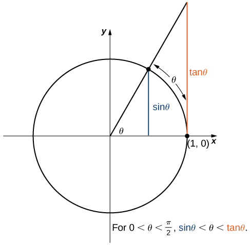
By dividing by \(\text{sin}\,θ\) in all parts of the inequality, we obtain
\[1<\frac{θ}{\text{sin}\,θ}<\frac{1}{\text{cos}\,θ}.\]
Equivalently, we have
\[1>\frac{\text{sin}\,θ}{θ}>\text{cos}\,θ.\]
Since \(\underset{θ\to {0}^{+}}{\text{lim}}1=1=\underset{θ\to {0}^{+}}{\text{lim}}\text{cos}\,θ,\) we conclude that \(\underset{θ\to {0}^{+}}{\text{lim}}\frac{\text{sin}\,θ}{θ}=1.\) By applying a manipulation similar to that used in demonstrating that \(\underset{θ\to {0}^{-}}{\text{lim}}\text{sin}\,θ=0,\) we can show that \(\underset{θ\to {0}^{-}}{\text{lim}}\frac{\text{sin}\,θ}{θ}=1.\) Thus,
\[\underset{θ\to 0}{\text{lim}}\frac{\text{sin}\,θ}{θ}=1.\]
In Example 13 we use this limit to establish \(\underset{θ\to 0}{\text{lim}}\frac{1-\text{cos}\,θ}{θ}=0.\) This limit also proves useful in later chapters.
Evaluate \(\underset{θ\to 0}{\text{lim}}\frac{1-\text{cos}\,θ}{θ}.\)
Multiply by the conjugate of 1−cos θ to bring in a sin²θ term and reuse the limit from just above.
In the first step, we multiply by the conjugate so that we can use a trigonometric identity to convert the cosine in the numerator to a sine:
\[\begin{array}{ll}\underset{θ\to 0}{\text{lim}}\frac{1-\text{cos}\,θ}{θ} & =\underset{θ\to 0}{\text{lim}}\frac{1-\text{cos}\,θ}{θ}·\frac{1+\text{cos}\,θ}{1+\text{cos}\,θ} \\ & =\underset{θ\to 0}{\text{lim}}\frac{1-{\text{cos}}^{2}θ}{θ(1+\text{cos}\,θ)} \\ & =\underset{θ\to 0}{\text{lim}}\frac{{\text{sin}}^{2}θ}{θ(1+\text{cos}\,θ)} \\ & =\underset{θ\to 0}{\text{lim}}\frac{\text{sin}\,θ}{θ}·\frac{\text{sin}\,θ}{1+\text{cos}\,θ} \\ & =1·\frac{0}{2}=0.\end{array}\]
Therefore,
\[\underset{θ\to 0}{\text{lim}}\frac{1-\text{cos}\,θ}{θ}=0.\]
Evaluate \(\underset{θ\to 0}{\text{lim}}\frac{1-\text{cos}\,θ}{\text{sin}\,θ}.\)
0
Some of the geometric formulas we take for granted today were first derived by methods that anticipate some of the methods of calculus. The Greek mathematician Archimedes (ca. 287−212; BCE) was particularly inventive, using polygons inscribed within circles to approximate the area of the circle as the number of sides of the polygon increased. He never came up with the idea of a limit, but we can use this idea to see what his geometric constructions could have predicted about the limit.
We can estimate the area of a circle by computing the area of an inscribed regular polygon. Think of the regular polygon as being made up of n triangles. By taking the limit as the vertex angle of these triangles goes to zero, you can obtain the area of the circle. To see this, carry out the following steps:
- Express the height h and the base b of the isosceles triangle in Figure 8 in terms of \(θ\) and r.
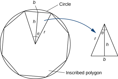
Figure 8 - Using the expressions that you obtained in step 1, express the area of the isosceles triangle in terms of θ and r.
(Substitute \((1\,\text{/}\,2)\,\text{sin}\,θ\) for \(\text{sin}(θ\,\text{/}\,2)\,\text{cos}(θ\,\text{/}\,2)\) in your expression.) - If an n-sided regular polygon is inscribed in a circle of radius r, find a relationship between θ and n. Solve this for n. Keep in mind there are 2π radians in a circle. (Use radians, not degrees.)
- Find an expression for the area of the n-sided polygon in terms of r and θ.
- To find a formula for the area of the circle, find the limit of the expression in step 4 as θ goes to zero. (Hint: \(\underset{θ\to 0}{\text{lim}}\frac{(\text{sin}\,θ)}{θ}=1\text{).}\)
The technique of estimating areas of regions by using polygons is revisited in Introduction to Integration.
Key Concepts
- The limit laws allow us to evaluate limits of functions without having to go through step-by-step processes each time.
- For polynomials and rational functions, \(\underset{x\to a}{\text{lim}}f(x)=f(a).\)
- You can evaluate the limit of a function by factoring and canceling, by multiplying by a conjugate, or by simplifying a complex fraction.
- The squeeze theorem allows you to find the limit of a function if the function is always greater than one function and less than another function with limits that are known.
Key Equations
| Basic Limit Results | \(\underset{x\to a}{\text{lim}}x=a\,\underset{x\to a}{\text{lim}}c=c\) |
| Important Limits | \(\underset{θ\to 0}{\text{lim}}\text{sin}\,θ=0\) \(\underset{θ\to 0}{\text{lim}}\text{cos}\,θ=1\) \(\underset{θ\to 0}{\text{lim}}\frac{\text{sin}\,θ}{θ}=1\) \(\underset{θ\to 0}{\text{lim}}\frac{1-\text{cos}\,θ}{θ}=0\) |
Section Exercises
In the following exercises, use the limit laws to evaluate each limit. Justify each step by indicating the appropriate limit law(s).
\(\underset{x\to 0}{\text{lim}}(4{x}^{2}-2x+3)\)
Use constant multiple law and difference law: \(\underset{x\to 0}{\text{lim}}(4{x}^{2}-2x+3)=4\underset{x\to 0}{\text{lim}}{x}^{2}-2\underset{x\to 0}{\text{lim}}x+\underset{x\to 0}{\text{lim}}3=3\)
\(\underset{x\to 1}{\text{lim}}\frac{{x}^{3}+3{x}^{2}+5}{4-7x}\)
\(\underset{x\to -2}{\text{lim}}\sqrt{{x}^{2}-6x+3}\)
Use root law: \(\underset{x\to -2}{\text{lim}}\sqrt{{x}^{2}-6x+3}=\sqrt{\underset{x\to -2}{\text{lim}}({x}^{2}-6x+3)}=\sqrt{19}\)
\(\underset{x\to -1}{\text{lim}}{(9x+1)}^{2}\)
In the following exercises, use direct substitution to evaluate each limit.
\(\underset{x\to 7}{\text{lim}}{x}^{2}\)
49
\(\underset{x\to -2}{\text{lim}}(4{x}^{2}-1)\)
\(\underset{x\to 0}{\text{lim}}\frac{1}{1+\text{sin}\,x}\)
1
\(\underset{x\to 2}{\text{lim}}{e}^{2x-{x}^{2}}\)
\(\underset{x\to 1}{\text{lim}}\frac{2-7x}{x+6}\)
\(-\frac{5}{7}\)
\(\underset{x\to 3}{\text{lim}}\text{ln}{e}^{3x}\)
In the following exercises, use direct substitution to show that each limit leads to the indeterminate form \(0\text{/}0.\) Then, evaluate the limit.
\(\underset{x\to 4}{\text{lim}}\frac{{x}^{2}-16}{x-4}\)
\(\underset{x\to 4}{\text{lim}}\frac{{x}^{2}-16}{x-4}=\frac{16-16}{4-4}=\frac{0}{0};\) then, \(\underset{x\to 4}{\text{lim}}\frac{{x}^{2}-16}{x-4}=\underset{x\to 4}{\text{lim}}\frac{(x+4)(x-4)}{x-4}=8\)
\(\underset{x\to 2}{\text{lim}}\frac{x-2}{{x}^{2}-2x}\)
\(\underset{x\to 6}{\text{lim}}\frac{3x-18}{2x-12}\)
\(\underset{x\to 6}{\text{lim}}\frac{3x-18}{2x-12}=\frac{18-18}{12-12}=\frac{0}{0};\) then, \(\underset{x\to 6}{\text{lim}}\frac{3x-18}{2x-12}=\underset{x\to 6}{\text{lim}}\frac{3(x-6)}{2(x-6)}=\frac{3}{2}\)
\(\underset{h\to 0}{\text{lim}}\frac{{(1+h)}^{2}-1}{h}\)
\(\underset{t\to 9}{\text{lim}}\frac{t-9}{\sqrt{t}-3}\)
\(\underset{x\to 9}{\text{lim}}\frac{t-9}{\sqrt{t}-3}=\frac{9-9}{3-3}=\frac{0}{0};\) then, \(\underset{t\to 9}{\text{lim}}\frac{t-9}{\sqrt{t}-3}=\underset{t\to 9}{\text{lim}}\frac{t-9}{\sqrt{t}-3}\frac{\sqrt{t}+3}{\sqrt{t}+3}=\underset{t\to 9}{\text{lim}}(\sqrt{t}+3)=6\)
\(\underset{h\to 0}{\text{lim}}\frac{\frac{1}{a+h}-\frac{1}{a}}{h},\) where a is a non-zero real-valued constant
\(\underset{θ\to \pi }{\text{lim}}\frac{\text{sin}\,θ}{\text{tan}\,θ}\)
\(\underset{θ\to \pi }{\text{lim}}\frac{\text{sin}\,θ}{\text{tan}\,θ}=\frac{\text{sin}\,\pi }{\text{tan}\,\pi }=\frac{0}{0};\) then, \(\underset{θ\to \pi }{\text{lim}}\frac{\text{sin}\,θ}{\text{tan}\,θ}=\underset{θ\to \pi }{\text{lim}}\frac{\text{sin}\,θ}{\frac{\text{sin}\,θ}{\text{cos}\,θ}}=\underset{θ\to \pi }{\text{lim}}\text{cos}\,θ=-1\)
\(\underset{x\to 1}{\text{lim}}\frac{{x}^{3}-1}{{x}^{2}-1}\)
\(\underset{x\to 1\text{/}2}{\text{lim}}\frac{2{x}^{2}+3x-2}{2x-1}\)
\(\underset{x\to 1\text{/}2}{\text{lim}}\frac{2{x}^{2}+3x-2}{2x-1}=\frac{\frac{1}{2}+\frac{3}{2}-2}{1-1}=\frac{0}{0};\) then, \(\underset{x\to 1\text{/}2}{\text{lim}}\frac{2{x}^{2}+3x-2}{2x-1}=\underset{x\to 1\text{/}2}{\text{lim}}\frac{(2x-1)(x+2)}{2x-1}=\frac{5}{2}\)
\(\underset{x\to -3}{\text{lim}}\frac{\sqrt{x+4}-1}{x+3}\)
In the following exercises, use direct substitution to obtain an undefined expression. Then, use the method of Example 11 to simplify the function to help determine the limit.
\(\underset{x\to {-2}^{-}}{\text{lim}}\frac{2{x}^{2}+7x-4}{{x}^{2}+x-2}\)
−∞
\(\underset{x\to {-2}^{+}}{\text{lim}}\frac{2{x}^{2}+7x-4}{{x}^{2}+x-2}\)
\(\underset{x\to {1}^{-}}{\text{lim}}\frac{2{x}^{2}+7x-4}{{x}^{2}+x-2}\)
−∞
\(\underset{x\to {1}^{+}}{\text{lim}}\frac{2{x}^{2}+7x-4}{{x}^{2}+x-2}\)
In the following exercises, assume that \(\underset{x\to 6}{\text{lim}}f(x)=4,\underset{x\to 6}{\text{lim}}g(x)=9,\) and \(\underset{x\to 6}{\text{lim}}h(x)=6.\) Use these three facts and the limit laws to evaluate each limit.
\(\underset{x\to 6}{\text{lim}}2f(x)g(x)\)
\(\underset{x\to 6}{\text{lim}}2f(x)g(x)=2\underset{x\to 6}{\text{lim}}f(x)\underset{x\to 6}{\text{lim}}g(x)=72\)
\(\underset{x\to 6}{\text{lim}}\frac{g(x)-1}{f(x)}\)
\(\underset{x\to 6}{\text{lim}}(f(x)+\frac{1}{3}g(x))\)
\(\underset{x\to 6}{\text{lim}}(f(x)+\frac{1}{3}g(x))=\underset{x\to 6}{\text{lim}}f(x)+\frac{1}{3}\underset{x\to 6}{\text{lim}}g(x)=7\)
\(\underset{x\to 6}{\text{lim}}\frac{{(h(x))}^{3}}{2}\)
\(\underset{x\to 6}{\text{lim}}\sqrt{g(x)-f(x)}\)
\(\underset{x\to 6}{\text{lim}}\sqrt{g(x)-f(x)}=\sqrt{\underset{x\to 6}{\text{lim}}g(x)-\underset{x\to 6}{\text{lim}}f(x)}=\sqrt{5}\)
\(\underset{x\to 6}{\text{lim}}x·h(x)\)
\(\underset{x\to 6}{\text{lim}}[(x+1)·f(x)]\)
\(\underset{x\to 6}{\text{lim}}[(x+1)f(x)]=(\underset{x\to 6}{\text{lim}}(x+1))(\underset{x\to 6}{\text{lim}}f(x))=28\)
\(\underset{x\to 6}{\text{lim}}(f(x)·g(x)-h(x))\)
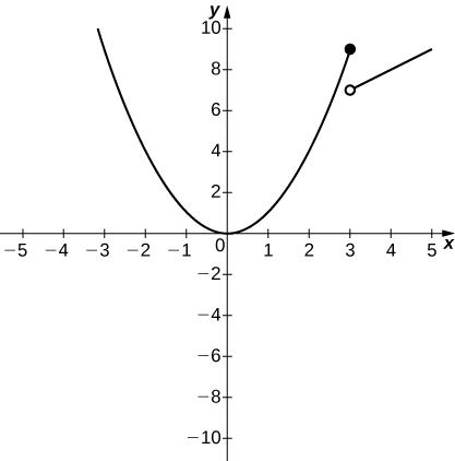
[T] In the following exercises, use a calculator to draw the graph of each piecewise-defined function and study the graph to evaluate the given limits.
\(f(x)=\left\{\begin{array}{ll}{x}^{2}, & x\le 3 \\ x+4, & x>3\end{array}\right.\)
- \(\underset{x\to {3}^{-}}{\text{lim}}f(x)\)
- \(\underset{x\to {3}^{+}}{\text{lim}}f(x)\)
3. There is an open circle at (3, 7), and the slope is 1.">
a. 9; b. 7
\(g(x)=\left\{\begin{array}{ll}{x}^{3}-1, & x\le 0 \\ 1, & x>0\end{array}\right.\)
- \(\underset{x\to {0}^{-}}{\text{lim}}g(x)\)
- \(\underset{x\to {0}^{+}}{\text{lim}}g(x)\)
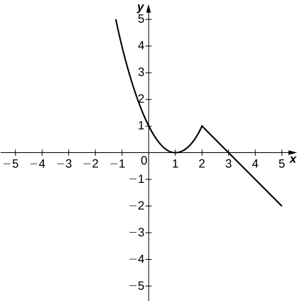
\(h(x)=\left\{\begin{array}{ll}{x}^{2}-2x+1, & x<2 \\ 3-x, & x\ge 2\end{array}\right.\)
- \(\underset{x\to {2}^{-}}{\text{lim}}h(x)\)
- \(\underset{x\to {2}^{+}}{\text{lim}}h(x)\)
= 2. It has a slope of -1 and an x intercept at (3,0).">
a. 1; b. 1
In the following exercises, use the following graphs and the limit laws to evaluate each limit.
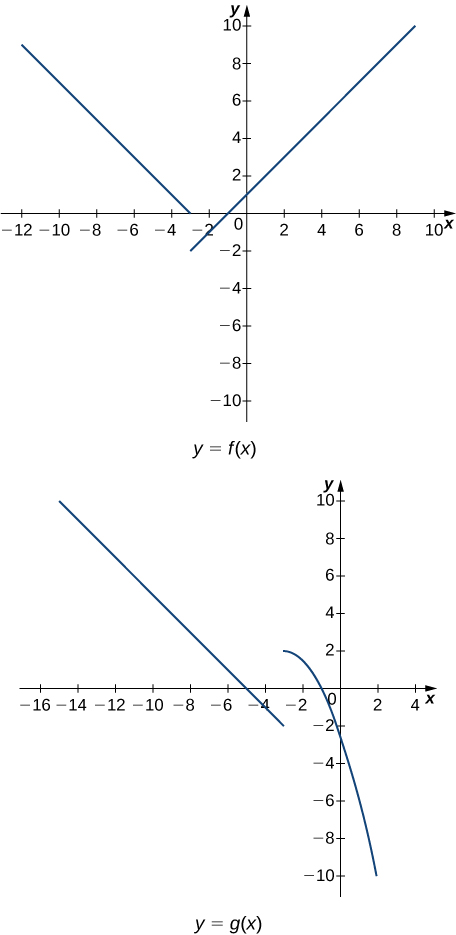
\(\underset{x\to {-3}^{+}}{\text{lim}}(f(x)+g(x))\)
\(\underset{x\to {-3}^{-}}{\text{lim}}(f(x)-3g(x))\)
\(\underset{x\to {-3}^{-}}{\text{lim}}(f(x)-3g(x))=\underset{x\to {-3}^{-}}{\text{lim}}f(x)-3\underset{x\to {-3}^{-}}{\text{lim}}g(x)=0+6=6\)
\(\underset{x\to 0}{\text{lim}}\frac{f(x)g(x)}{3}\)
\(\underset{x\to -5}{\text{lim}}\frac{2+g(x)}{f(x)}\)
\(\underset{x\to -5}{\text{lim}}\frac{2+g(x)}{f(x)}=\frac{2+(\underset{x\to -5}{\text{lim}}g(x))}{\underset{x\to -5}{\text{lim}}f(x)}=\frac{2+0}{2}=1\)
\(\underset{x\to 1}{\text{lim}}{(f(x))}^{2}\)
\(\underset{x\to 1}{\text{lim}}\sqrt[3]{f(x)-g(x)}\)
\(\underset{x\to 1}{\text{lim}}\sqrt[3]{f(x)-g(x)}=\sqrt[3]{\underset{x\to 1}{\text{lim}}f(x)-\underset{x\to 1}{\text{lim}}g(x)}=\sqrt[3]{2+5}=\sqrt[3]{7}\)
\(\underset{x\to -7}{\text{lim}}(x·g(x))\)
\(\underset{x\to -9}{\text{lim}}[x·f(x)+2·g(x)]\)
\(\underset{x\to -9}{\text{lim}}(xf(x)+2g(x))=(\underset{x\to -9}{\text{lim}}x)(\underset{x\to -9}{\text{lim}}f(x))+2\underset{x\to -9}{\text{lim}}(g(x))=(-9)(6)+2(4)=-46\)
For the following problems, evaluate the limit using the squeeze theorem. Use a calculator to graph the functions \(f(x),g(x),\) and \(h(x)\) when possible.
[T] True or False? If \(2x-1\le g(x)\le {x}^{2}-2x+3,\) then \(\underset{x\to 2}{\text{lim}}g(x)=0.\)
[T] \(\underset{θ\to 0}{\text{lim}}{θ}^{2}\text{cos}\,(\frac{1}{θ})\)
The limit is zero.
![The graph of three functions over the domain [-1,1], colored red, green, and blue as follows: red: theta^2, green: theta^2 * cos (1/theta), and blue: - (theta^2). The red and blue functions open upwards and downwards respectively as parabolas with vertices at the origin. The green function is trapped between the two.](https://raw.githubusercontent.com/openstax/osbooks-calculus-bundle/main/media/CNX_Calc_Figure_02_03_206.jpg)
\(\underset{x\to 0}{\text{lim}}f(x),\) where \(f(x)=\left\{\begin{array}{ll}0, & x\,\text{rational} \\ {x}^{2}, & x\,\text{irrational}\end{array}\right.\)
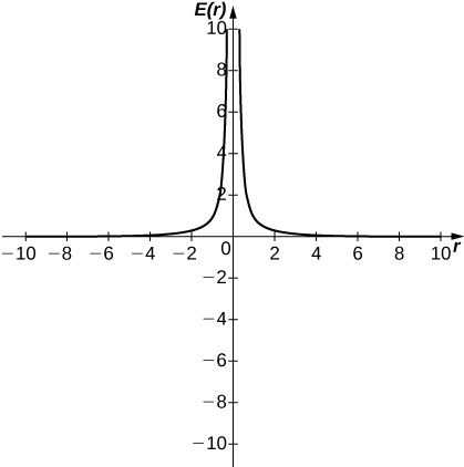
[T] In physics, the magnitude of an electric field generated by a point charge at a distance r in vacuum is governed by Coulomb’s law: \(E(r)=\frac{q}{4\pi {ε}_{0}{r}^{2}},\) where E represents the magnitude of the electric field, q is the charge of the particle, r is the distance between the particle and where the strength of the field is measured, and \(\frac{1}{4\pi {ε}_{0}}\) is Coulomb’s constant: \(8.988\,\times \,{10}^{9}\,\text{N}·{\text{m}}^{2}\text{/}{\text{C}}^{2}.\)
- Use a graphing calculator to graph \(E(r)\) given that the charge of the particle is \(q={10}^{-10}.\)
- Evaluate \(\underset{r\to {0}^{+}}{\text{lim}}E(r).\) What is the physical meaning of this quantity? Is it physically relevant? Why are you evaluating from the right?
a.
b. ∞. The magnitude of the electric field as you approach the particle q becomes infinite. It does not make physical sense to evaluate negative distance.
[T] The density of an object is given by its mass divided by its volume: \(ρ=m\text{/}V.\)
- Use a calculator to plot the volume as a function of density \((V=m\text{/}ρ),\) assuming you are examining something of mass 8 kg ( \(m=8\text{).}\)
- Evaluate \(\underset{ρ\to {0}^{+}}{\text{lim}}V(ρ)\) and explain the physical meaning.
Glossary
- constant multiple law for limits
- the limit law \(\underset{x\to a}{\text{lim}}cf(x)=c·\underset{x\to a}{\text{lim}}f(x)=cL\)
- difference law for limits
- the limit law \(\underset{x\to a}{\text{lim}}(f(x)-g(x))=\underset{x\to a}{\text{lim}}f(x)-\underset{x\to a}{\text{lim}}g(x)=L-M\)
- limit laws
- the individual properties of limits; for each of the individual laws, let \(f(x)\) and \(g(x)\) be defined for all \(x\ne a\) over some open interval containing a; assume that L and M are real numbers so that \(\underset{x\to a}{\text{lim}}f(x)=L\) and \(\underset{x\to a}{\text{lim}}g(x)=M;\) let c be a constant
- power law for limits
- the limit law \(\underset{x\to a}{\text{lim}}{(f(x))}^{n}={(\underset{x\to a}{\text{lim}}f(x))}^{n}={L}^{n}\) for every positive integer n
- product law for limits
- the limit law \(\underset{x\to a}{\text{lim}}(f(x)·g(x))=\underset{x\to a}{\text{lim}}f(x)·\underset{x\to a}{\text{lim}}g(x)=L·M\)
- quotient law for limits
- the limit law \(\underset{x\to a}{\text{lim}}\frac{f(x)}{g(x)}=\frac{\underset{x\to a}{\text{lim}}f(x)}{\underset{x\to a}{\text{lim}}g(x)}=\frac{L}{M}\) for \(M\ne 0\)
- root law for limits
- the limit law \(\underset{x\to a}{\text{lim}}\sqrt[n]{f(x)}=\sqrt[n]{\underset{x\to a}{\text{lim}}f(x)}=\sqrt[n]{L}\) for all L if n is odd and for \(L\ge 0\) if n is even
- squeeze theorem
- states that if \(f(x)\le g(x)\le h(x)\) for all \(x\ne a\) over an open interval containing a and \(\underset{x\to a}{\text{lim}}f(x)=L=\underset{x\to a}{\text{lim}}h(x)\) where L is a real number, then \(\underset{x\to a}{\text{lim}}g(x)=L\)
- sum law for limits
- The limit law \(\underset{x\to a}{\text{lim}}(f(x)+g(x))=\underset{x\to a}{\text{lim}}f(x)+\underset{x\to a}{\text{lim}}g(x)=L+M\)