Section 2.2The Limit of a Function
The concept of a limit or limiting process, essential to the understanding of calculus, has been around for thousands of years. In fact, early mathematicians used a limiting process to obtain better and better approximations of areas of circles. Yet, the formal definition of a limit—as we know and understand it today—did not appear until the late 19th century. We therefore begin our quest to understand limits, as our mathematical ancestors did, by using an intuitive approach. At the end of this chapter, armed with a conceptual understanding of limits, we examine the formal definition of a limit.
We begin our exploration of limits by taking a look at the graphs of the functions
\[f(x)=\frac{{x}^{2}-4}{x-2},\,g(x)=\frac{\text{|}x-2\text{|}}{x-2},\,\text{and}\,h(x)=\frac{1}{{(x-2)}^{2}},\]
which are shown in Figure 1. In particular, let’s focus our attention on the behavior of each graph at and around \(x=2.\)
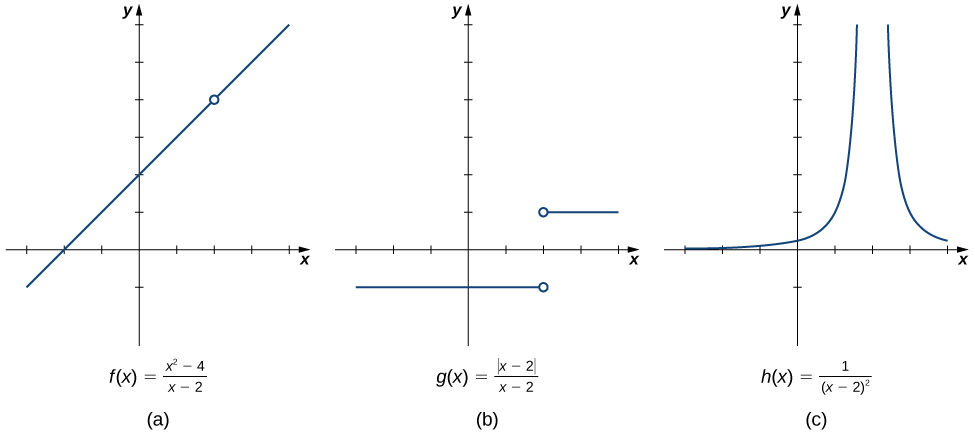
Each of the three functions is undefined at \(x=2,\) but if we make this statement and no other, we give a very incomplete picture of how each function behaves in the vicinity of \(x=2.\) To express the behavior of each graph in the vicinity of 2 more completely, we need to introduce the concept of a limit.
Intuitive Definition of a Limit
Let’s first take a closer look at how the function \(f(x)=({x}^{2}-4)\text{/}(x-2)\) behaves around \(x=2\) in Figure 1. As the values of x approach 2 from either side of 2, the values of \(y=f(x)\) approach 4. Mathematically, we say that the limit of \(f(x)\) as x approaches 2 is 4. Symbolically, we express this limit as
\[\underset{x\to 2}{\text{lim}}f(x)=4.\]
From this very brief informal look at one limit, let’s start to develop an intuitive definition of the limit. We can think of the limit of a function at a number a as being the one real number L that the functional values approach as the x-values approach a, provided such a real number L exists. Stated more carefully, we have the following definition:
Let \(f(x)\) be a function defined at all values in an open interval containing a, with the possible exception of a itself, and let L be a real number. If all values of the function \(f(x)\) approach the real number L as the values of \(x(\ne a)\) approach the number a, then we say that the limit of \(f(x)\) as x approaches a is L. (More succinct, as x gets closer to a, \(f(x)\) gets closer and stays close to L.) Symbolically, we express this idea as
\[\underset{x\to a}{\text{lim}}f(x)=L.\]
We can estimate limits by constructing tables of functional values and by looking at their graphs. This process is described in the following Problem-Solving Strategy.
- To evaluate \(\underset{x\to a}{\text{lim}}f(x),\) we begin by completing a table of functional values. We should choose two sets of x-values—one set of values approaching a and less than a, and another set of values approaching a and greater than a. Table 1 demonstrates what your tables might look like.
Table 1 x \(f(x)\) x \(f(x)\) \(a-0.1\) \(f(a-0.1)\) \(a+0.1\) \(f(a+0.1)\) \(a-0.01\) \(f(a-0.01)\) \(a+0.01\) \(f(a+0.01)\) \(a-0.001\) \(f(a-0.001)\) \(a+0.001\) \(f(a+0.001)\) \(a-0.0001\) \(f(a-0.0001)\) \(a+0.0001\) \(f(a+0.0001)\) Use additional values as necessary. Use additional values as necessary. - Next, let’s look at the values in each of the \(f(x)\) columns and determine whether the values seem to be approaching a single value as we move down each column. In our columns, we look at the sequence \(f(a-0.1),f(a-0.01),f(a-0.001).,f(a-0.0001),\) and so on, and \(f(a+0.1),f(a+0.01),f(a+0.001),f(a+0.0001),\) and so on. (Note: Although we have chosen the x-values \(a\pm 0.1,a\pm 0.01,a\pm 0.001,a\pm 0.0001,\) and so forth, and these values will probably work nearly every time, on very rare occasions we may need to modify our choices.)
- If both columns approach a common y-value L, we state \(\underset{x\to a}{\text{lim}}f(x)=L.\) We can use the following strategy to confirm the result obtained from the table or as an alternative method for estimating a limit.
- Using a graphing calculator or computer software that allows us to graph functions, we can plot the function \(f(x),\) making sure the functional values of \(f(x)\) for x-values near a are in our window. We can use the trace feature to move along the graph of the function and watch the y-value readout as the x-values approach a. If the y-values approach L as our x-values approach a from both directions, then \(\underset{x\to a}{\text{lim}}f(x)=L.\) We may need to zoom in on our graph and repeat this process several times.
We apply this Problem-Solving Strategy to compute a limit in Example 1.
Evaluate \(\underset{x\to 0}{\text{lim}}\frac{\text{sin}\,x}{x}\) using a table of functional values.
Build the table with x-values approaching 0 from both sides — the pattern in the outputs is the limit.
We have calculated the values of \(f(x)=(\text{sin}\,x)\text{/}x\) for the values of x listed in Table 2.
| x | \(\frac{\text{sin}\,x}{x}\) | x | \(\frac{\text{sin}\,x}{x}\) | |
| −0.1 | 0.998334166468 | 0.1 | 0.998334166468 | |
| −0.01 | 0.999983333417 | 0.01 | 0.999983333417 | |
| −0.001 | 0.999999833333 | 0.001 | 0.999999833333 | |
| −0.0001 | 0.999999998333 | 0.0001 | 0.999999998333 |
Note: The values in this table were obtained using a calculator and using all the places given in the calculator output.
As we read down each \(\frac{(\text{sin}\,x)}{x}\) column, we see that the values in each column appear to be approaching one. Thus, it is fairly reasonable to conclude that \(\underset{x\to 0}{\text{lim}}\frac{\text{sin}\,x}{x}=1.\) A calculator or computer-generated graph of \(f(x)=\frac{(\text{sin}\,x)}{x}\) would be similar to that shown in Figure 2, and it confirms our estimate.
![A graph of f(x) = sin(x)/x over the interval [-6, 6]. The curving function has a y intercept at x=0 and x intercepts at y=pi and y=-pi.](https://raw.githubusercontent.com/openstax/osbooks-calculus-bundle/main/media/CNX_Calc_Figure_02_02_003.jpg)
Evaluate \(\underset{x\to 4}{\text{lim}}\frac{\sqrt{x}-2}{x-4}\) using a table of functional values.
Same table strategy as Example 1 — this time approach x=4 from both sides.
As before, we use a table—in this case, Table 3—to list the values of the function for the given values of x.
| x | \(\frac{\sqrt{x}-2}{x-4}\) | x | \(\frac{\sqrt{x}-2}{x-4}\) | |
| 3.9 | 0.251582341869 | 4.1 | 0.248456731317 | |
| 3.99 | 0.25015644562 | 4.01 | 0.24984394501 | |
| 3.999 | 0.250015627 | 4.001 | 0.249984377 | |
| 3.9999 | 0.250001563 | 4.0001 | 0.249998438 | |
| 3.99999 | 0.25000016 | 4.00001 | 0.24999984 |
After inspecting this table, we see that the functional values less than 4 appear to be decreasing toward 0.25 whereas the functional values greater than 4 appear to be increasing toward 0.25. We conclude that \(\underset{x\to 4}{\text{lim}}\frac{\sqrt{x}-2}{x-4}=0.25.\) We confirm this estimate using the graph of \(f(x)=\frac{\sqrt{x}-2}{x-4}\) shown in Figure 3.
![A graph of the function f(x) = (sqrt(x) – 2 ) / (x-4) over the interval [0,8]. There is an open circle on the function at x=4. The function curves asymptotically towards the x axis and y axis in quadrant one.](https://raw.githubusercontent.com/openstax/osbooks-calculus-bundle/main/media/CNX_Calc_Figure_02_02_004.jpg)
Estimate \(\underset{x\to 1}{\text{lim}}\frac{\frac{1}{x}-1}{x-1}\) using a table of functional values. Use a graph to confirm your estimate.
Same table approach as before — approach x=1 from both sides.
\(\underset{x\to 1}{\text{lim}}\frac{\frac{1}{x}-1}{x-1}=-1\)
At this point, we see from Example 1 and Example 2 that it may be just as easy, if not easier, to estimate a limit of a function by inspecting its graph as it is to estimate the limit by using a table of functional values. In Example 3, we evaluate a limit exclusively by looking at a graph rather than by using a table of functional values.
For \(g(x)\) shown in Figure 4, evaluate \(\underset{x\to -1}{\text{lim}}g(x).\)
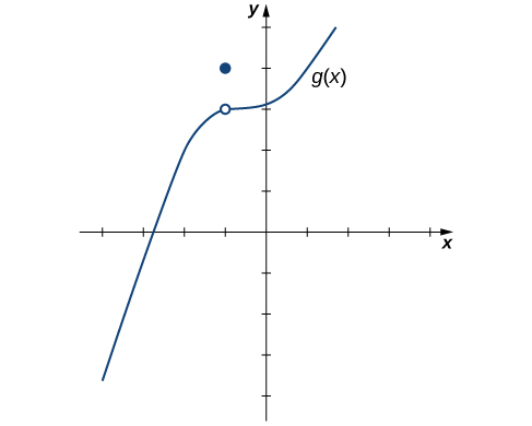
Read the y-value the curve approaches near x=−1 — the single point off the curve doesn't matter.
Despite the fact that \(g(-1)=4,\) as the x-values approach −1 from either side, the \(g(x)\) values approach 3. Therefore, \(\underset{x\to -1}{\text{lim}}g(x)=3.\) Note that we can determine this limit without even knowing the algebraic expression of the function.
Based on Example 3, we make the following observation: It is possible for the limit of a function to exist at a point, and for the function to be defined at this point, but the limit of the function and the value of the function at the point may be different.
Use the graph of \(h(x)\) in Figure 5 to evaluate \(\underset{x\to 2}{\text{lim}}h(x),\) if possible.
![A graph of the function h(x), which is a parabola graphed over [-2.5, 5]. There is an open circle where the vertex should be at the point (2,-1).](https://raw.githubusercontent.com/openstax/osbooks-calculus-bundle/main/media/CNX_Calc_Figure_02_02_007.jpg)
Same idea as Example 3 — the missing point at the vertex doesn't change what the curve approaches.
\(\underset{x\to 2}{\text{lim}}h(x)=-1.\)
Looking at a table of functional values or looking at the graph of a function provides us with useful insight into the value of the limit of a function at a given point. However, these techniques rely too much on guesswork. We eventually need to develop alternative methods of evaluating limits. These new methods are more algebraic in nature and we explore them in the next section; however, at this point we introduce two special limits that are foundational to the techniques to come.
Let a be a real number and c be a constant.
\[\underset{x\to a}{\text{lim}}x=a\]
\[\underset{x\to a}{\text{lim}}c=c\]
We can make the following observations about these two limits.
- For the first limit, observe that as x approaches a, so does \(f(x),\) because \(f(x)=x.\) Consequently, \(\underset{x\to a}{\text{lim}}x=a.\)
- For the second limit, consider Table 4.
| x | \(f(x)=c\) | x | \(f(x)=c\) | |
| \(a-0.1\) | c | \(a+0.1\) | c | |
| \(a-0.01\) | c | \(a+0.01\) | c | |
| \(a-0.001\) | c | \(a+0.001\) | c | |
| \(a-0.0001\) | c | \(a+0.0001\) | c |
Observe that for all values of x (regardless of whether they are approaching a), the values \(f(x)\) remain constant at c. We have no choice but to conclude \(\underset{x\to a}{\text{lim}}c=c.\)
The Existence of a Limit
As we consider the limit in the next example, keep in mind that for the limit of a function to exist at a point, the functional values must approach a single real-number value at that point. If the functional values do not approach a single value, then the limit does not exist.
Evaluate \(\underset{x\to 0}{\text{lim}}\text{sin}\,(1\text{/}\text{x})\) using a table of values.
Watch what happens as the table values get very close to 0 — the oscillation is the key here.
Table 5 lists values for the function \(\text{sin}(1\text{/}x)\) for the given values of x.
| x | \(\text{sin}(\frac{1}{x})\) | x | \(\text{sin}(\frac{1}{x})\) | |
| −0.1 | 0.544021110889 | 0.1 | −0.544021110889 | |
| −0.01 | 0.50636564111 | 0.01 | −0.50636564111 | |
| −0.001 | −0.8268795405312 | 0.001 | 0.826879540532 | |
| −0.0001 | 0.305614388888 | 0.0001 | −0.305614388888 | |
| −0.00001 | −0.035748797987 | 0.00001 | 0.035748797987 | |
| −0.000001 | 0.349993504187 | 0.000001 | −0.349993504187 |
After examining the table of functional values, we can see that the y-values do not seem to approach any one single value. It appears the limit does not exist. Before drawing this conclusion, let’s take a more systematic approach. Take the following sequence of x-values approaching 0:
\[\frac{2}{\pi },\frac{2}{3\pi },\frac{2}{5\pi },\frac{2}{7\pi },\frac{2}{9\pi },\frac{2}{11\pi }\text{,….}\]
The corresponding y-values are
\[1,-1,1,-1,1,-1\text{,….}\]
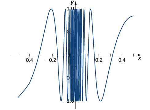
At this point we can indeed conclude that \(\underset{x\to 0}{\text{lim}}\text{sin}\,(1\text{/}\text{x})\) does not exist. (Mathematicians frequently abbreviate “does not exist” as DNE. Thus, we would write \(\underset{x\to 0}{\text{lim}}\text{sin}\,(1\text{/}\text{x})\) DNE.) The graph of \(f(x)=\text{sin}\,(1\text{/}x)\) is shown in Figure 6 and it gives a clearer picture of the behavior of \(\text{sin}(1\text{/}x)\) as x approaches 0. You can see that \(\text{sin}(1\text{/}\text{x})\) oscillates ever more wildly between −1 and 1 as x approaches 0.
Use a table of functional values to evaluate \(\underset{x\to 2}{\text{lim}}\frac{\text{|}{x}^{2}-4\text{|}}{x-2},\) if possible.
Build the table as before — compare the left- and right-approaching values before combining.
\(\underset{x\to 2}{\text{lim}}\frac{\text{|}{x}^{2}-4\text{|}}{x-2}\) does not exist.
One-Sided Limits
Sometimes indicating that the limit of a function fails to exist at a point does not provide us with enough information about the behavior of the function at that particular point. To see this, we now revisit the function \(g(x)=\text{|}x-2\text{|}\text{/}(x-2)\) introduced at the beginning of the section (see Figure 1(b)). As we pick values of x close to 2, \(g(x)\) does not approach a single value, so the limit as x approaches 2 does not exist—that is, \(\underset{x\to 2}{\text{lim}}g(x)\) DNE. However, this statement alone does not give us a complete picture of the behavior of the function around the x-value 2. To provide a more accurate description, we introduce the idea of a one-sided limit. For all values to the left of 2 (or the negative side of 2), \(g(x)=-1.\) Thus, as x approaches 2 from the left, \(g(x)\) approaches −1. Mathematically, we say that the limit as x approaches 2 from the left is −1. Symbolically, we express this idea as
\[\underset{x\to {2}^{-}}{\text{lim}}g(x)=-1.\]
Similarly, as x approaches 2 from the right (or from the positive side), \(g(x)\) approaches 1. Symbolically, we express this idea as
\[\underset{x\to {2}^{+}}{\text{lim}}g(x)=1.\]
We can now present an informal definition of one-sided limits.
We define two types of one-sided limits.
Limit from the left: Let \(f(x)\) be a function defined at all values in an open interval of the form (c, a), and let L be a real number. If the values of the function \(f(x)\) approach the real number L as the values of x (where \(x<\text{a}\text{)}\) approach the number a, then we say that L is the limit of \(f(x)\) as x approaches a from the left. Symbolically, we express this idea as
\[\underset{x\to {a}^{-}}{\text{lim}}f(x)=L.\]
Limit from the right: Let \(f(x)\) be a function defined at all values in an open interval of the form \((a,c),\) and let L be a real number. If the values of the function \(f(x)\) approach the real number L as the values of x (where \(x>\text{a}\text{)}\) approach the number a, then we say that L is the limit of \(f(x)\) as x approaches a from the right. Symbolically, we express this idea as
\[\underset{x\to {a}^{+}}{\text{lim}}f(x)=L.\]
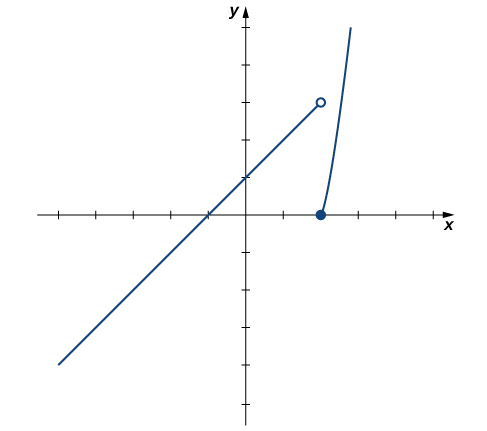
For the function \(f(x)=\left\{\begin{array}{ll}x+1 & \text{if}\,x<2 \\ {x}^{2}-4 & \text{if}\,x\ge 2\end{array}\right.,\) evaluate each of the following limits.
- \(\underset{x\to {2}^{-}}{\text{lim}}f(x)\)
- \(\underset{x\to {2}^{+}}{\text{lim}}f(x)\)
Evaluate the left piece as x→2⁻ and the right piece as x→2⁺ separately, then compare.
We can use tables of functional values again Table 6. Observe that for values of x less than 2, we use \(f(x)=x+1\) and for values of x greater than 2, we use \(f(x)={x}^{2}-4.\)
| x | \(f(x)=x+1\) | x | \(f(x)={x}^{2}-4\) | |
| 1.9 | 2.9 | 2.1 | 0.41 | |
| 1.99 | 2.99 | 2.01 | 0.0401 | |
| 1.999 | 2.999 | 2.001 | 0.004001 | |
| 1.9999 | 2.9999 | 2.0001 | 0.00040001 | |
| 1.99999 | 2.99999 | 2.00001 | 0.0000400001 |
Based on this table, we can conclude that a. \(\underset{x\to {2}^{-}}{\text{lim}}f(x)=3\) and b. \(\underset{x\to {2}^{+}}{\text{lim}}f(x)=0.\) Therefore, the (two-sided) limit of \(f(x)\) does not exist at \(x=2.\) Figure 7 shows a graph of \(f(x)\) and reinforces our conclusion about these limits.
Use a table of functional values to estimate the following limits, if possible.
- \(\underset{x\to {2}^{-}}{\text{lim}}\frac{\text{|}{x}^{2}-4\text{|}}{x-2}\)
- \(\underset{x\to {2}^{+}}{\text{lim}}\frac{\text{|}{x}^{2}-4\text{|}}{x-2}\)
Same piecewise idea as Example 5 — check each one-sided limit before combining.
a. \(\underset{x\to {2}^{-}}{\text{lim}}\frac{\text{|}{x}^{2}-4\text{|}}{x-2}=-4;\) b. \(\underset{x\to {2}^{+}}{\text{lim}}\frac{\text{|}{x}^{2}-4\text{|}}{x-2}=4\)
Let us now consider the relationship between the limit of a function at a point and the limits from the right and left at that point. It seems clear that if the limit from the right and the limit from the left have a common value, then that common value is the limit of the function at that point. Similarly, if the limit from the left and the limit from the right take on different values, the limit of the function does not exist. These conclusions are summarized in the theorem below.
Let \(f(x)\) be a function defined at all values in an open interval containing a, with the possible exception of a itself, and let L be a real number. Then,
\[\underset{x\to a}{\text{lim}}f(x)=L\,\text{if and only if}\,\underset{x\to {a}^{-}}{\text{lim}}f(x)=L\,\text{and}\,\underset{x\to {a}^{+}}{\text{lim}}f(x)=L.\]
Infinite Limits
Evaluating the limit of a function at a point or evaluating the limit of a function from the right and left at a point helps us to characterize the behavior of a function around a given value. As we shall see, we can also describe the behavior of functions that do not have finite limits.
We now turn our attention to \(h(x)=1\text{/}{(x-2)}^{2},\) the third and final function introduced at the beginning of this section (see Figure 1(c)). From its graph we see that as the values of x approach 2, the values of \(h(x)=1\text{/}{(x-2)}^{2}\) become larger and larger and, in fact, become infinite. Mathematically, we say that the limit of \(h(x)\) as x approaches 2 is positive infinity. Symbolically, we express this idea as
\[\underset{x\to 2}{\text{lim}}h(x)=\text{+}\infty .\]
More generally, we define infinite limits as follows:
We define three types of infinite limits.
Infinite limits from the left: Let \(f(x)\) be a function defined at all values in an open interval of the form \((b,a).\)
- If the values of \(f(x)\) increase without bound as the values of x (where \(x<\text{a}\text{)}\) approach the number a, then we say that the limit as x approaches a from the left is positive infinity and we write
\[\underset{x\to {a}^{-}}{\text{lim}}f(x)=\text{+}\infty .\]
- If the values of \(f(x)\) decrease without bound as the values of x (where \(x<\text{a}\text{)}\) approach the number a, then we say that the limit as x approaches a from the left is negative infinity and we write
\[\underset{x\to {a}^{-}}{\text{lim}}f(x)=\text{-}\infty .\]
Infinite limits from the right: Let \(f(x)\) be a function defined at all values in an open interval of the form \((a,c).\)
- If the values of \(f(x)\) increase without bound as the values of x (where \(x>\text{a}\text{)}\) approach the number a, then we say that the limit as x approaches a from the right is positive infinity and we write
\[\underset{x\to {a}^{+}}{\text{lim}}f(x)=\text{+}\infty .\]
- If the values of \(f(x)\) decrease without bound as the values of x (where \(x>\text{a}\text{)}\) approach the number a, then we say that the limit as x approaches a from the right is negative infinity and we write
\[\underset{x\to {a}^{+}}{\text{lim}}f(x)=\text{-}\infty .\]
Two-sided infinite limit: Let \(f(x)\) be defined for all \(x\ne a\) in an open interval containing a.
- If the values of \(f(x)\) increase without bound as the values of x (where \(x\ne \text{a}\text{)}\) approach the number a, then we say that the limit as x approaches a is positive infinity and we write
\[\underset{x\to a}{\text{lim}}f(x)=\text{+}\infty .\]
- If the values of \(f(x)\) decrease without bound as the values of x (where \(x\ne \text{a}\text{)}\) approach the number a, then we say that the limit as x approaches a is negative infinity and we write
\[\underset{x\to a}{\text{lim}}f(x)=\text{-}\infty .\]
It is important to understand that when we write statements such as \(\underset{x\to a}{\text{lim}}f(x)=\text{+}\infty\) or \(\underset{x\to a}{\text{lim}}f(x)=\text{-}\infty\) we are describing the behavior of the function, as we have just defined it. We are not asserting that a limit exists. For the limit of a function \(f(x)\) to exist at a, it must approach a real number L as x approaches a. That said, if, for example, \(\underset{x\to a}{\text{lim}}f(x)=\text{+}\infty ,\) we always write \(\underset{x\to a}{\text{lim}}f(x)=\text{+}\infty\) rather than \(\underset{x\to a}{\text{lim}}f(x)\) DNE.
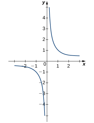
Evaluate each of the following limits, if possible. Use a table of functional values and graph \(f(x)=1\text{/}x\) to confirm your conclusion.
- \(\underset{x\to {0}^{-}}{\text{lim}}\frac{1}{x}\)
- \(\underset{x\to {0}^{+}}{\text{lim}}\frac{1}{x}\)
- \(\underset{x\to 0}{\text{lim}}\frac{1}{x}\)
Track the sign of 1/x as x approaches 0 from each side.
Begin by constructing a table of functional values.
| x | \(\frac{1}{x}\) | x | \(\frac{1}{x}\) | |
| −0.1 | −10 | 0.1 | 10 | |
| −0.01 | −100 | 0.01 | 100 | |
| −0.001 | −1000 | 0.001 | 1000 | |
| −0.0001 | −10,000 | 0.0001 | 10,000 | |
| −0.00001 | −100,000 | 0.00001 | 100,000 | |
| −0.000001 | −1,000,000 | 0.000001 | 1,000,000 |
- The values of \(1\text{/}x\) decrease without bound as x approaches 0 from the left. We conclude that
\[\underset{x\to {0}^{-}}{\text{lim}}\frac{1}{x}=\text{-}\infty .\]
- The values of \(1\text{/}x\) increase without bound as x approaches 0 from the right. We conclude that
\[\underset{x\to {0}^{+}}{\text{lim}}\frac{1}{x}=\text{+}\infty .\]
- Since \(\underset{x\to {0}^{-}}{\text{lim}}\frac{1}{x}=\text{-}\infty\) and \(\underset{x\to {0}^{+}}{\text{lim}}\frac{1}{x}=\text{+}\infty\) have different values, we conclude that
\[\underset{x\to 0}{\text{lim}}\frac{1}{x}\,\text{DNE.}\]
The graph of \(f(x)=1\text{/}x\) in Figure 8 confirms these conclusions.
Evaluate each of the following limits, if possible. Use a table of functional values and graph \(f(x)=1\text{/}{x}^{2}\) to confirm your conclusion.
- \(\underset{x\to {0}^{-}}{\text{lim}}\frac{1}{{x}^{2}}\)
- \(\underset{x\to {0}^{+}}{\text{lim}}\frac{1}{{x}^{2}}\)
- \(\underset{x\to 0}{\text{lim}}\frac{1}{{x}^{2}}\)
Same idea as Example 6, but with 1/x² both sides now push the same direction.
a. \(\underset{x\to {0}^{-}}{\text{lim}}\frac{1}{{x}^{2}}=\text{+}\infty ;\) b. \(\underset{x\to {0}^{+}}{\text{lim}}\frac{1}{{x}^{2}}=\text{+}\infty ;\) c. \(\underset{x\to 0}{\text{lim}}\frac{1}{{x}^{2}}=\text{+}\infty\)
It is useful to point out that functions of the form \(f(x)=1\text{/}{(x-a)}^{n},\) where n is a positive integer, have infinite limits as x approaches a from either the left or right (Figure 9). These limits are summarized in the theorem below.
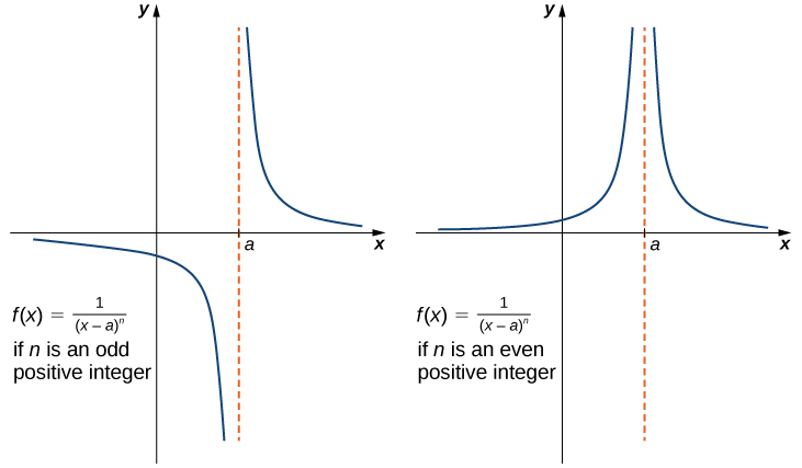
If n is a positive even integer, then
\[\underset{x\to a}{\text{lim}}\frac{1}{{(x-a)}^{n}}=\text{+}\infty .\]
If n is a positive odd integer, then
\[\underset{x\to {a}^{+}}{\text{lim}}\frac{1}{{(x-a)}^{n}}=\text{+}\infty \]
and
\[\underset{x\to {a}^{-}}{\text{lim}}\frac{1}{{(x-a)}^{n}}=\text{-}\infty .\]
We should also point out that in the graphs of \(f(x)=1\text{/}{(x-a)}^{n},\) points on the graph having x-coordinates very near to a are very close to the vertical line \(x=a.\) That is, as x approaches a, the points on the graph of \(f(x)\) are closer to the line \(x=a.\) The line \(x=a\) is called a vertical asymptote of the graph. We formally define a vertical asymptote as follows:
Let \(f(x)\) be a function. If any of the following conditions hold, then the line \(x=a\) is a vertical asymptote of \(f(x).\)
\[\begin{array}{lll}\underset{x\to {a}^{-}}{\text{lim}}f(x) & = & \text{+}\infty \,\text{or}\,\text{-∞} \\ \underset{x\to {a}^{+}}{\text{lim}}f(x) & = & \text{+}\infty \,\text{or}\,\text{-∞} \\ & \,\text{or} & \\ \underset{x\to a}{\text{lim}}f(x) & = & \text{+}\infty \,\text{or}\,\text{-∞}\end{array}\]
Evaluate each of the following limits using the theorem above. Identify any vertical asymptotes of the function \(f(x)=1\text{/}{(x+3)}^{4}.\)
- \(\underset{x\to {-3}^{-}}{\text{lim}}\frac{1}{{(x+3)}^{4}}\)
- \(\underset{x\to {-3}^{+}}{\text{lim}}\frac{1}{{(x+3)}^{4}}\)
- \(\underset{x\to -3}{\text{lim}}\frac{1}{{(x+3)}^{4}}\)
Apply the theorem above directly — check whether the exponent is even or odd.
We can use the theorem above directly.
- \(\underset{x\to {-3}^{-}}{\text{lim}}\frac{1}{{(x+3)}^{4}}=\text{+}\infty\)
- \(\underset{x\to {-3}^{+}}{\text{lim}}\frac{1}{{(x+3)}^{4}}=\text{+}\infty\)
- \(\underset{x\to -3}{\text{lim}}\frac{1}{{(x+3)}^{4}}=\text{+}\infty\)
The function \(f(x)=1\text{/}{(x+3)}^{4}\) has a vertical asymptote of \(x=-3.\)
Evaluate each of the following limits. Identify any vertical asymptotes of the function \(f(x)=\frac{1}{{(x-2)}^{3}}.\)
- \(\underset{x\to {2}^{-}}{\text{lim}}\frac{1}{{(x-2)}^{3}}\)
- \(\underset{x\to {2}^{+}}{\text{lim}}\frac{1}{{(x-2)}^{3}}\)
- \(\underset{x\to 2}{\text{lim}}\frac{1}{{(x-2)}^{3}}\)
Same theorem as Example 7, but with an odd exponent — the two one-sided limits will disagree in sign.
a. \(\underset{x\to {2}^{-}}{\text{lim}}\frac{1}{{(x-2)}^{3}}=\text{-}\infty ;\) b. \(\underset{x\to {2}^{+}}{\text{lim}}\frac{1}{{(x-2)}^{3}}=\text{+}\infty ;\) c. \(\underset{x\to 2}{\text{lim}}\frac{1}{{(x-2)}^{3}}\) DNE. The line \(x=2\) is the vertical asymptote of \(f(x)=1\text{/}{(x-2)}^{3}.\)
In the next example we put our knowledge of various types of limits to use to analyze the behavior of a function at several different points.
Use the graph of \(f(x)\) in Figure 10 to determine each of the following values:
- \(\underset{x\to {-4}^{-}}{\text{lim}}f(x);\underset{x\to {-4}^{+}}{\text{lim}}f(x);\underset{x\to -4}{\text{lim}}f(x);f(-4)\)
- \(\underset{x\to {-2}^{-}}{\text{lim}}f(x);\underset{x\to {-2}^{+}}{\text{lim}}f(x);\underset{x\to -2}{\text{lim}}f(x);f(-2)\)
- \(\underset{x\to {1}^{-}}{\text{lim}}f(x);\underset{x\to {1}^{+}}{\text{lim}}f(x);\underset{x\to 1}{\text{lim}}f(x);f(1)\)
- \(\underset{x\to {3}^{-}}{\text{lim}}f(x);\underset{x\to {3}^{+}}{\text{lim}}f(x);\underset{x\to 3}{\text{lim}}f(x);f(3)\)
![The graph of a function f(x) described by the above limits and values. There is a smooth curve for values below x=-2; at (-2, 3), there is an open circle. There is a smooth curve between (-2, 1] with a closed circle at (1,6). There is an open circle at (1,3), and a smooth curve stretching from there down asymptotically to negative infinity along x=3. The function also curves asymptotically along x=3 on the other side, also stretching to negative infinity. The function then changes concavity in the first quadrant around y=4.5 and continues up.](https://raw.githubusercontent.com/openstax/osbooks-calculus-bundle/main/media/CNX_Calc_Figure_02_02_015.jpg)
Read each one-sided limit directly off the graph at each x-value, then compare to the function value.
Using the one-sided/two-sided limits theorem and the graph for reference, we arrive at the following values:
- \(\underset{x\to {-4}^{-}}{\text{lim}}f(x)=0;\underset{x\to {-4}^{+}}{\text{lim}}f(x)=0;\underset{x\to -4}{\text{lim}}f(x)=0;f(-4)=0\)
- \(\underset{x\to {-2}^{-}}{\text{lim}}f(x)=3.;\underset{x\to {-2}^{+}}{\text{lim}}f(x)=3;\underset{x\to -2}{\text{lim}}f(x)=3;f(-2)\) is undefined
- \(\underset{x\to {1}^{-}}{\text{lim}}f(x)=6;\underset{x\to {1}^{+}}{\text{lim}}f(x)=3;\underset{x\to 1}{\text{lim}}f(x)\) DNE; \(f(1)=6\)
- \(\underset{x\to {3}^{-}}{\text{lim}}f(x)=\text{-}\infty ;\underset{x\to {3}^{+}}{\text{lim}}f(x)=\text{-}\infty ;\underset{x\to 3}{\text{lim}}f(x)=\text{-}\infty ;f(3)\) is undefined
Evaluate \(\underset{x\to 1}{\text{lim}}f(x)\) for \(f(x)\) shown here:
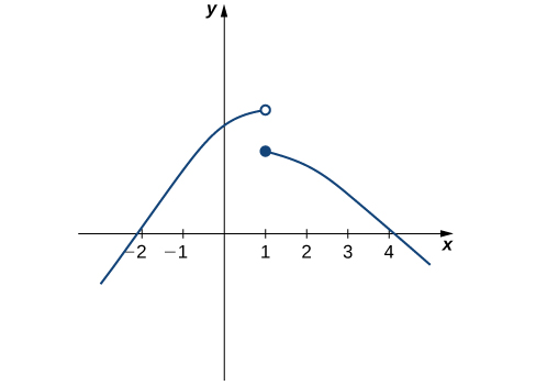
Same graph-reading approach as Example 8 — check both sides of x=1 before combining.
Does not exist.
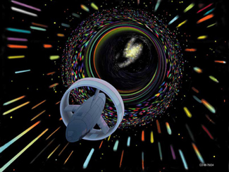
In the chapter opener we mentioned briefly how Albert Einstein showed that a limit exists to how fast any object can travel. Given Einstein’s equation for the mass of a moving object, what is the value of this bound?
Plug values of v/c approaching 1 into the mass formula and watch what happens to the denominator.
Our starting point is Einstein’s equation for the mass of a moving object,
\[m=\frac{{m}_{0}}{\sqrt{1-\frac{{v}^{2}}{{c}^{2}}}},\]
where \({m}_{0}\) is the object’s mass at rest, v is its speed, and c is the speed of light. To see how the mass changes at high speeds, we can graph the ratio of masses \(m\text{/}{m}_{0}\) as a function of the ratio of speeds, \(v\text{/}c\) (Figure 12).
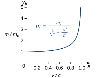
We can see that as the ratio of speeds approaches 1—that is, as the speed of the object approaches the speed of light—the ratio of masses increases without bound. In other words, the function has a vertical asymptote at \(v\text{/}c=1.\) We can try a few values of this ratio to test this idea.
| \(\frac{v}{c}\) | \(\sqrt{1-\frac{{v}^{2}}{{c}^{2}}}\) | \(\frac{m}{{m}_{0}}\) |
| 0.99 | 0.1411 | 7.089 |
| 0.999 | 0.0447 | 22.37 |
| 0.9999 | 0.0141 | 70.71 |
Thus, according to Table 8, if an object with mass 100 kg is traveling at 0.9999c, its mass becomes 7071 kg. Since no object can have an infinite mass, we conclude that no object can travel at or more than the speed of light.
Key Concepts
- A table of values or graph may be used to estimate a limit.
- If the limit of a function at a point does not exist, it is still possible that the limits from the left and right at that point may exist.
- If the limits of a function from the left and right exist and are equal, then the limit of the function is that common value.
- We may use limits to describe infinite behavior of a function at a point.
Key Equations
| Intuitive Definition of the Limit | \(\underset{x\to a}{\text{lim}}f(x)=L\) |
| Two Important Limits | \(\underset{x\to a}{\text{lim}}x=a\,\underset{x\to a}{\text{lim}}c=c\) |
| One-Sided Limits | \(\underset{x\to {a}^{-}}{\text{lim}}f(x)=L\,\underset{x\to {a}^{+}}{\text{lim}}f(x)=L\) |
| Infinite Limits from the Left | \(\underset{x\to {a}^{-}}{\text{lim}}f(x)=\text{+}\infty \,\underset{x\to {a}^{-}}{\text{lim}}f(x)=\text{-}\infty\) |
| Infinite Limits from the Right | \(\underset{x\to {a}^{+}}{\text{lim}}f(x)=\text{+}\infty \,\underset{x\to {a}^{+}}{\text{lim}}f(x)=\text{-}\infty\) |
| Two-Sided Infinite Limits | \(\underset{x\to a}{\text{lim}}f(x)=\text{+}\infty :\underset{x\to {a}^{-}}{\text{lim}}f(x)=\text{+}\infty\) and \(\underset{x\to {a}^{+}}{\text{lim}}f(x)=\text{+}\infty\) \(\underset{x\to a}{\text{lim}}f(x)=\text{-}\infty :\underset{x\to {a}^{-}}{\text{lim}}f(x)=\text{-}\infty\) and \(\underset{x\to {a}^{+}}{\text{lim}}f(x)=\text{-}\infty\) |
Section Exercises
For the following exercises, consider the function \(f(x)=\frac{{x}^{2}-1}{\text{|}x-1\text{|}}.\)
[T] Complete the following table for the function. Round your solutions to four decimal places.
| x | \(f(x)\) | x | \(f(x)\) | |
| 0.9 | a. | 1.1 | e. | |
| 0.99 | b. | 1.01 | f. | |
| 0.999 | c. | 1.001 | g. | |
| 0.9999 | d. | 1.0001 | h. |
What do your results in the preceding exercise indicate about the two-sided limit \(\underset{x\to 1}{\text{lim}}f(x)?\) Explain your response.
\(\underset{x\to 1}{\text{lim}}f(x)\) does not exist because \(\underset{x\to {1}^{-}}{\text{lim}}f(x)=-2\ne \underset{x\to {1}^{+}}{\text{lim}}f(x)=2.\)
For the following exercises, consider the function \(f(x)={(1+x)}^{1\text{/}x}.\)
[T] Make a table showing the values of f for \(x=-0.01,-0.001,-0.0001,-0.00001\) and for \(x=0.01,0.001,0.0001,0.00001.\) Round your solutions to five decimal places.
| x | \(f(x)\) | x | \(f(x)\) | |
| −0.01 | a. | 0.01 | e. | |
| −0.001 | b. | 0.001 | f. | |
| −0.0001 | c. | 0.0001 | g. | |
| −0.00001 | d. | 0.00001 | h. |
What does the table of values in the preceding exercise indicate about the function \(f(x)={(1+x)}^{1\text{/}x}?\)
\(\underset{x\to 0}{\text{lim}}{(1+x)}^{1\text{/}x}=2.7183\)
To which mathematical constant does the limit in the preceding exercise appear to be getting closer?
In the following exercises, use the given values to set up a table to evaluate the limits. Round your solutions to eight decimal places.
[T] \(\underset{x\to 0}{\text{lim}}\frac{\text{sin}\,2x}{x};\,\pm 0.1,\pm 0.01,\pm 0.001,\pm .0001\)
| x | \(\frac{\text{sin}\,2x}{x}\) | x | \(\frac{\text{sin}\,2x}{x}\) | |
| −0.1 | a. | 0.1 | e. | |
| −0.01 | b. | 0.01 | f. | |
| −0.001 | c. | 0.001 | g. | |
| −0.0001 | d. | 0.0001 | h. |
a. 1.98669331; b. 1.99986667; c. 1.99999867; d. 1.99999999; e. 1.98669331; f. 1.99986667; g. 1.99999867; h. 1.99999999; \(\underset{x\to 0}{\text{lim}}\frac{\text{sin}\,2x}{x}=2\)
[T] \(\underset{x\to 0}{\text{lim}}\frac{\text{sin}\,3x}{x}\) ±0.1, ±0.01, ±0.001, ±0.0001
| X | \(\frac{\text{sin}\,3x}{x}\) | x | \(\frac{\text{sin}\,3x}{x}\) | |
| −0.1 | a. | 0.1 | e. | |
| −0.01 | b. | 0.01 | f. | |
| −0.001 | c. | 0.001 | g. | |
| −0.0001 | d. | 0.0001 | h. |
Use the preceding two exercises to conjecture (guess) the value of the following limit: \(\underset{x\to 0}{\text{lim}}\frac{\text{sin}\,ax}{x}\) for a, a positive real value.
\(\underset{x\to 0}{\text{lim}}\frac{\text{sin}\,ax}{x}=a\)
[T] In the following exercises, set up a table of values to find the indicated limit. Round to eight digits.
\(\underset{x\to 2}{\text{lim}}\frac{{x}^{2}-4}{{x}^{2}+x-6}\)
| x | \(\frac{{x}^{2}-4}{{x}^{2}+x-6}\) | x | \(\frac{{x}^{2}-4}{{x}^{2}+x-6}\) | |
| 1.9 | a. | 2.1 | e. | |
| 1.99 | b. | 2.01 | f. | |
| 1.999 | c. | 2.001 | g. | |
| 1.9999 | d. | 2.0001 | h. |
\(\underset{x\to 1}{\text{lim}}(1-2x)\)
| x | \(1-2x\) | x | \(1-2x\) | |
| 0.9 | a. | 1.1 | e. | |
| 0.99 | b. | 1.01 | f. | |
| 0.999 | c. | 1.001 | g. | |
| 0.9999 | d. | 1.0001 | h. |
a. −0.80000000; b. −0.98000000; c. −0.99800000; d. −0.99980000; e. −1.2000000; f. −1.0200000; g. −1.0020000; h. −1.0002000; \(\underset{x\to 1}{\text{lim}}(1-2x)=-1\)
\(\underset{x\to 0}{\text{lim}}\frac{5}{1-{e}^{1\text{/}x}}\)
| x | \(\frac{5}{1-{e}^{1\text{/}x}}\) | x | \(\frac{5}{1-{e}^{1\text{/}x}}\) | |
| −0.1 | a. | 0.1 | e. | |
| −0.01 | b. | 0.01 | f. | |
| −0.001 | c. | 0.001 | g. | |
| −0.0001 | d. | 0.0001 | h. |
\(\underset{z\to 0}{\text{lim}}\frac{z-1}{{z}^{2}(z+3)}\)
| z | \(\frac{z-1}{{z}^{2}(z+3)}\) | z | \(\frac{z-1}{{z}^{2}(z+3)}\) | |
| −0.1 | a. | 0.1 | e. | |
| −0.01 | b. | 0.01 | f. | |
| −0.001 | c. | 0.001 | g. | |
| −0.0001 | d. | 0.0001 | h. |
a. −37.931934; b. −3377.9264; c. −333,777.93; d. −33,337,778; e. −29.032258; f. −3289.0365; g. −332,889.04; h. −33,328,889 \(\underset{x\to 0}{\text{lim}}\frac{z-1}{{z}^{2}(z+3)}=\text{-}\infty\)
\(\underset{t\to {0}^{+}}{\text{lim}}\frac{\text{cos}\,t}{t}\)
| t | \(\frac{\text{cos}\,t}{t}\) |
| 0.1 | a. |
| 0.01 | b. |
| 0.001 | c. |
| 0.0001 | d. |
\(\underset{x\to 2}{\text{lim}}\frac{1-\frac{2}{x}}{{x}^{2}-4}\)
| x | \(\frac{1-\frac{2}{x}}{{x}^{2}-4}\) | x | \(\frac{1-\frac{2}{x}}{{x}^{2}-4}\) | |
| 1.9 | a. | 2.1 | e. | |
| 1.99 | b. | 2.01 | f. | |
| 1.999 | c. | 2.001 | g. | |
| 1.9999 | d. | 2.0001 | h. |
a. 0.13495277; b. 0.12594300; c. 0.12509381; d. 0.12500938; e. 0.11614402; f. 0.12406794; g. 0.12490631; h. 0.12499063; \(∴\underset{x\to 2}{\text{lim}}\frac{1-\frac{2}{x}}{{x}^{2}-4}=0.1250=\frac{1}{8}\)
[T] In the following exercises, set up a table of values and round to eight significant digits. Based on the table of values, make a guess about what the limit is. Then, use a calculator to graph the function and determine the limit. Was the conjecture correct? If not, why does the method of tables fail?
\(\underset{θ\to 0}{\text{lim}}\text{sin}\,(\frac{\pi }{θ})\)
| θ | \(\text{sin}\,(\frac{\pi }{θ})\) | θ | \(\text{sin}\,(\frac{\pi }{θ})\) | |
| −0.1 | a. | 0.1 | e. | |
| −0.01 | b. | 0.01 | f. | |
| −0.001 | c. | 0.001 | g. | |
| −0.0001 | d. | 0.0001 | h. |
\(\underset{α\to {0}^{+}}{\text{lim}}\frac{1}{α}\,\text{cos}\,(\frac{\pi }{α})\)
| \(α\) | \(\frac{1}{α}\,\text{cos}\,(\frac{\pi }{α})\) |
| 0.1 | a. |
| 0.01 | b. |
| 0.001 | c. |
| 0.0001 | d. |
a. 10.00000; b. 100.00000; c. 1000.0000; d. 10,000.000; Guess: \(\underset{α\to {0}^{+}}{\text{lim}}\frac{1}{α}\,\text{cos}\,(\frac{\pi }{α})=\infty ,\) actual: DNE
![A graph of the function (1/alpha) * cos (pi / alpha), which oscillates gently until the interval [-.2, .2], where it oscillates rapidly, going to infinity and negative infinity as it approaches the y axis.](https://raw.githubusercontent.com/openstax/osbooks-calculus-bundle/main/media/CNX_Calc_Figure_02_02_214.jpg)
In the following exercises, consider the graph of the function \(y=f(x)\) shown here. Which of the statements about \(y=f(x)\) are true and which are false? Explain why a statement is false.
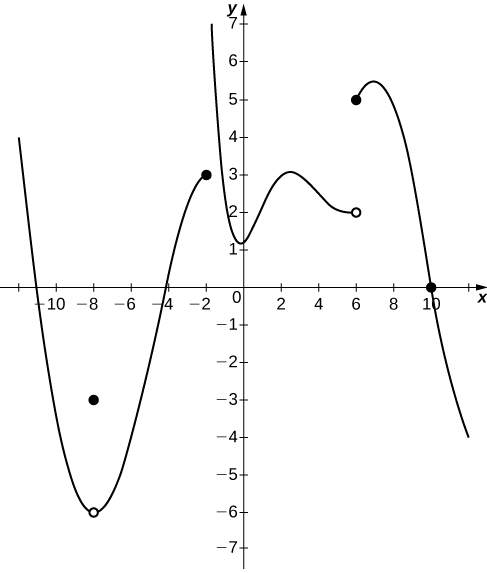
\(\underset{x\to 10}{\text{lim}}f(x)=0\)
\(\underset{x\to {-2}^{+}}{\text{lim}}f(x)=3\)
False; \(\underset{x\to {-2}^{+}}{\text{lim}}f(x)=\text{+}\infty\)
\(\underset{x\to -8}{\text{lim}}f(x)=f(-8)\)
\(\underset{x\to 6}{\text{lim}}f(x)=5\)
False; \(\underset{x\to 6}{\text{lim}}f(x)\) DNE since \(\underset{x\to {6}^{-}}{\text{lim}}f(x)=2\) and \(\underset{x\to {6}^{+}}{\text{lim}}f(x)=5.\)
In the following exercises, use the following graph of the function \(y=f(x)\) to find the values, if possible. Estimate when necessary.
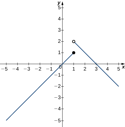
\(\underset{x\to {1}^{-}}{\text{lim}}f(x)\)
\(\underset{x\to {1}^{+}}{\text{lim}}f(x)\)
2
\(\underset{x\to 1}{\text{lim}}f(x)\)
\(\underset{x\to 2}{\text{lim}}f(x)\)
1
\(f(1)\)
In the following exercises, use the graph of the function \(y=f(x)\) shown here to find the values, if possible. Estimate when necessary.
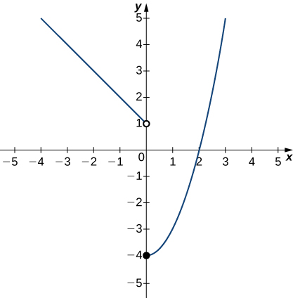
\(\underset{x\to {0}^{-}}{\text{lim}}f(x)\)
1
\(\underset{x\to {0}^{+}}{\text{lim}}f(x)\)
\(\underset{x\to 0}{\text{lim}}f(x)\)
DNE
\(\underset{x\to 2}{\text{lim}}f(x)\)
In the following exercises, use the graph of the function \(y=f(x)\) shown here to find the values, if possible. Estimate when necessary.
![A graph of a piecewise function with three segments, all linear. The first exists for x < -2, has a slope of 1, and ends at the open circle at (-2, 0). The second exists over the interval [-2, 2], has a slope of -1, goes through the origin, and has closed circles at its endpoints (-2, 2) and (2,-2). The third exists for x>2, has a slope of 1, and begins at the open circle (2,2).](https://raw.githubusercontent.com/openstax/osbooks-calculus-bundle/main/media/CNX_Calc_Figure_02_02_204.jpg)
\(\underset{x\to {-2}^{-}}{\text{lim}}f(x)\)
0
\(\underset{x\to {-2}^{+}}{\text{lim}}f(x)\)
\(\underset{x\to -2}{\text{lim}}f(x)\)
DNE
\(\underset{x\to {2}^{-}}{\text{lim}}f(x)\)
\(\underset{x\to {2}^{+}}{\text{lim}}f(x)\)
2
\(\underset{x\to 2}{\text{lim}}f(x)\)
In the following exercises, use the graph of the function \(y=g(x)\) shown here to find the values, if possible. Estimate when necessary.
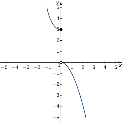
\(\underset{x\to {0}^{-}}{\text{lim}}g(x)\)
3
\(\underset{x\to {0}^{+}}{\text{lim}}g(x)\)
\(\underset{x\to 0}{\text{lim}}g(x)\)
DNE
In the following exercises, use the graph of the function \(y=h(x)\) shown here to find the values, if possible. Estimate when necessary.
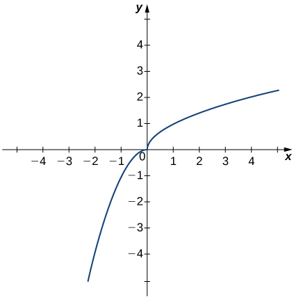
\(\underset{x\to {0}^{-}}{\text{lim}}h(x)\)
\(\underset{x\to {0}^{+}}{\text{lim}}h(x)\)
0
\(\underset{x\to 0}{\text{lim}}h(x)\)
In the following exercises, use the graph of the function \(y=f(x)\) shown here to find the values, if possible. Estimate when necessary.
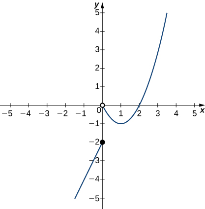
\(\underset{x\to {0}^{-}}{\text{lim}}f(x)\)
−2
\(\underset{x\to {0}^{+}}{\text{lim}}f(x)\)
\(\underset{x\to 0}{\text{lim}}f(x)\)
DNE
\(\underset{x\to 1}{\text{lim}}f(x)\)
\(\underset{x\to 2}{\text{lim}}f(x)\)
0
In the following exercises, sketch the graph of a function with the given properties.
\(\underset{x\to 2}{\text{lim}}f(x)=1,\underset{x\to {4}^{-}}{\text{lim}}f(x)=3,\underset{x\to {4}^{+}}{\text{lim}}f(x)=6,f(4)\) is not defined.
\(As x\to {-\infty} , f(x)\to 0,\underset{x\to {-1}^{-}}{\text{lim}}f(x)=\text{-}\infty ,\) \(\underset{x\to {-1}^{+}}{\text{lim}}f(x)=\infty ,\underset{x\to 0}{\text{lim}}f(x)=f(0),f(0)=1, As x\to \infty , f(x)\to \text{-}\infty\)
Answers may vary.
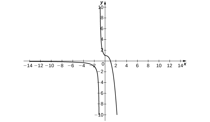
\(As x\to {-\infty} , f(x)\to 2,\underset{x\to {3}^{-}}{\text{lim}}f(x)=\text{-}\infty ,\) \(\underset{x\to {3}^{+}}{\text{lim}}f(x)=\infty , As x\to \infty , f(x)\to 2,f(0)=\frac{-1}{3}\)
\(As x\to {-\infty} , f(x)\to 2,\underset{x\to -2}{\text{lim}}f(x)=\text{-}\infty ,\) \(As x\to \infty , f(x)\to 2,f(0)=0\)
Answers may vary.
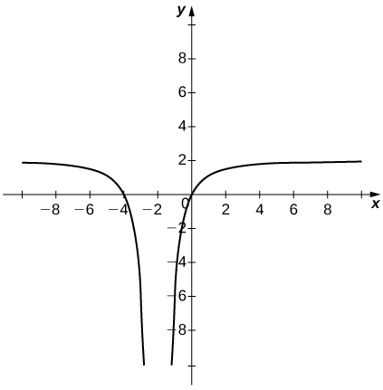
\(As x\to {-\infty} , f(x)\to 0,\underset{x\to {-1}^{-}}{\text{lim}}f(x)=\infty ,\underset{x\to {-1}^{+}}{\text{lim}}f(x)=\text{-}\infty ,\) \(f(0)=-1,\underset{x\to {1}^{-}}{\text{lim}}f(x)=\text{-}\infty ,\underset{x\to {1}^{+}}{\text{lim}}f(x)=\infty , As x\to \infty , f(x)\to 0\)
Shock waves arise in many physical applications, ranging from supernovas to detonation waves. A graph of the density of a shock wave with respect to distance, x, is shown here. We are mainly interested in the location of the front of the shock, labeled \({x}_{\text{SF}}\) in the diagram.
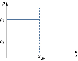
- Evaluate \(\underset{x\to {x}_{SF}{}^{+}}{\text{lim}}ρ(x).\)
- Evaluate \(\underset{x\to {x}_{SF}{}^{-}}{\text{lim}}ρ(x).\)
- Evaluate \(\underset{x\to {x}_{SF}}{\text{lim}}ρ(x).\) Explain the physical meanings behind your answers.
a. \({ρ}_{2}\) b. \({ρ}_{1}\) c. DNE unless \({ρ}_{1}={ρ}_{2}.\) As you approach \({x}_{\text{SF}}\) from the left, you are in the high-density area of the shock. When you approach from the right, you have not experienced the “shock” yet and are at a lower density.
A track coach uses a camera with a fast shutter to estimate the position of a runner with respect to time. A table of the values of position of the athlete versus time is given here, where x is the position in meters of the runner and t is time in seconds. What is \(\underset{t\to 2}{\text{lim}}x(t)?\) What does it mean physically?
| t (sec) | x (m) |
| 1.75 | 4.5 |
| 1.95 | 6.1 |
| 1.99 | 6.42 |
| 2.01 | 6.58 |
| 2.05 | 6.9 |
| 2.25 | 8.5 |
Glossary
- infinite limit
- A function has an infinite limit at a point a if it either increases or decreases without bound as it approaches a
- intuitive definition of the limit
- If all values of the function \(f(x)\) approach the real number L as the values of \(x(\ne a)\) approach a, \(f(x)\) approaches L
- one-sided limit
- A one-sided limit of a function is a limit taken from either the left or the right
- vertical asymptote
- A function has a vertical asymptote at \(x=a\) if the limit as x approaches a from the right or left is infinite