Section 7.4Series Solutions of Differential Equations
In Introduction to Power Series, we studied how functions can be represented as power series, \(y(x)=\sum_{n=0}^{\infty} {a}_{n}{x}^{n}.\) We also saw that we can find series representations of the derivatives of such functions by differentiating the power series term by term. This gives \({y}^{\prime }(x)=\sum_{n=1}^{\infty} n{a}_{n}{x}^{n-1}\) and \({y}^{\prime\prime }(x)=\sum_{n=2}^{\infty} n(n-1){a}_{n}{x}^{n-2}.\) In some cases, these power series representations can be used to find solutions to differential equations.
Be aware that this subject is given only a very brief treatment in this text. Most introductory differential equations textbooks include an entire chapter on power series solutions. This text has only a single section on the topic, so several important issues are not addressed here, particularly issues related to existence of solutions. The examples and exercises in this section were chosen for which power solutions exist. However, it is not always the case that power solutions exist. Those of you interested in a more rigorous treatment of this topic should consult a differential equations text.
- Assume the differential equation has a solution of the form \(y(x)=\sum_{n=0}^{\infty} {a}_{n}{x}^{n}.\)
- Differentiate the power series term by term to get \({y}^{\prime }(x)=\sum_{n=1}^{\infty} n{a}_{n}{x}^{n-1}\) and \({y}^{\prime\prime }(x)=\sum_{n=2}^{\infty} n(n-1){a}_{n}{x}^{n-2}.\)
- Substitute the power series expressions into the differential equation.
- Re-index sums as necessary to combine terms and simplify the expression.
- Equate coefficients of like powers of \(x\) to determine values for the coefficients \({a}_{n}\) in the power series.
- Substitute the coefficients back into the power series and write the solution.
Find a power series solution for the following differential equations.
- \({y}^{\prime\prime }-y=0\)
- \(({x}^{2}-1){y}^{\prime\prime }+6x{y}^{\prime }+4y=-4\)
Assume a solution \(y(x)=\sum a_nx^n,\) differentiate term by term to get \(y'\) and \(y'',\) substitute into the equation, and re-index the sums so every term has the same power of x before comparing coefficients.
- Assume \(y(x)=\sum_{n=0}^{\infty} {a}_{n}{x}^{n}\) (step 1). Then, \({y}^{\prime }(x)=\sum_{n=1}^{\infty} n{a}_{n}{x}^{n-1}\) and \({y}^{\prime\prime }(x)=\sum_{n=2}^{\infty} n(n-1){a}_{n}{x}^{n-2}\) (step 2). We want to find values for the coefficients \({a}_{n}\) such that
We want the indices on our sums to match so that we can express them using a single summation. That is, we want to rewrite the first summation so that it starts with \(n=0.\)
To re-index the first term, replace n with \(n+2\) inside the sum, and change the lower summation limit to \(n=0.\) We get
This gives
Because power series expansions of functions are unique, this equation can be true only if the coefficients of each power of x are zero. So we have
This recurrence relationship allows us to express each coefficient \({a}_{n}\) in terms of the coefficient two terms earlier. This yields one expression for even values of n and another expression for odd values of n. Looking first at the equations involving even values of n, we see that
Thus, in general, when n is even, \({a}_{n}=\frac{{a}_{0}}{n!}\) (step 5).
For the equations involving odd values of n, we see that
Therefore, in general, when n is odd, \({a}_{n}=\frac{{a}_{1}}{n!}\) (step 5 continued).
Putting this together, we have
Re-indexing the sums to account for the even and odd values of n separately, we obtain
Analysis for part a.
As expected for a second-order differential equation, this solution depends on two arbitrary constants. However, note that our differential equation is a constant-coefficient differential equation, yet the power series solution does not appear to have the familiar form (containing exponential functions) that we are used to seeing. Furthermore, since \(y(x)={c}_{1}{e}^{x}+{c}_{2}{e}^{\text{-}x}\) is the general solution to this equation, we must be able to write any solution in this form, and it is not clear whether the power series solution we just found can, in fact, be written in that form.
Fortunately, after writing the power series representations of \({e}^{x}\) and \({e}^{\text{-}x},\) and doing some algebra, we find that if we choose
we then have \({a}_{0}={c}_{0}+{c}_{1}\) and \({a}_{1}={c}_{0}-{c}_{1},\) and
So we have, in fact, found the same general solution. Note that this choice of \({c}_{1}\) and \({c}_{2}\) is not obvious. This is a case when we know what the answer should be, and have essentially “reverse-engineered” our choice of coefficients.\[\begin{array}{lll}{y}^{\prime\prime }-y & = & 0 \\ \sum_{n=2}^{\infty} n(n-1){a}_{n}{x}^{n-2}-\sum_{n=0}^{\infty} {a}_{n}{x}^{n} & = & 0\,\text{(step 3).}\end{array}\]
\[\sum_{n=2}^{\infty} n(n-1){a}_{n}{x}^{n-2}=\sum_{n=0}^{\infty} (n+2)(n+1){a}_{n+2}{x}^{n}.\]
\[\begin{array}{lll}\sum_{n=0}^{\infty} (n+2)(n+1){a}_{n+2}{x}^{n}-\sum_{n=0}^{\infty} {a}_{n}{x}^{n} & = & 0 \\ \sum_{n=0}^{\infty} [(n+2)(n+1){a}_{n+2}-{a}_{n}]{x}^{n} & = & 0\,\text{(step 4).}\end{array}\]
\[(n+2)(n+1){a}_{n+2}-{a}_{n}=0\,\text{for}\,n=0,1,2\text{,….}\]
\[\begin{array}{lll}{a}_{2} & = & \frac{{a}_{0}}{2} \\ {a}_{4} & = & \frac{{a}_{2}}{4\cdot 3}=\frac{{a}_{0}}{4!} \\ {a}_{6} & = & \frac{{a}_{4}}{6\cdot 5}=\frac{{a}_{0}}{6!} \\ & \vdots. & \end{array}\]
\[\begin{array}{lll}{a}_{3} & = & \frac{{a}_{1}}{3\cdot 2}=\frac{{a}_{1}}{3!} \\ {a}_{5} & = & \frac{{a}_{3}}{5\cdot 4}=\frac{{a}_{1}}{5!} \\ {a}_{7} & = & \frac{{a}_{5}}{7\cdot 6}=\frac{{a}_{1}}{7!} \\ & \vdots. & \end{array}\]
\[\begin{array}{ll}y(x) & =\sum_{n=0}^{\infty} {a}_{n}{x}^{n} \\ & ={a}_{0}+{a}_{1}x+\frac{{a}_{0}}{2}{x}^{2}+\frac{{a}_{1}}{3!}{x}^{3}+\frac{{a}_{0}}{4!}{x}^{4}+\frac{{a}_{1}}{5!}{x}^{5}+\cdots \text{.}\end{array}\]
\[y(x)={a}_{0}\sum_{k=0}^{\infty} \frac{1}{(2k)!}{x}^{2k}+{a}_{1}\sum_{k=0}^{\infty} \frac{1}{(2k+1)!}{x}^{2k+1}\,\text{(step 6).}\]
\[{c}_{0}=\frac{({a}_{0}+{a}_{1})}{2},\,{c}_{1}=\frac{({a}_{0}-{a}_{1})}{2},\]
\[\begin{array}{ll}y(x) & ={a}_{0}+{a}_{1}x+\frac{{a}_{0}}{2}{x}^{2}+\frac{{a}_{1}}{3!}{x}^{3}+\frac{{a}_{0}}{4!}{x}^{4}+\frac{{a}_{1}}{5!}{x}^{5}+\cdots \\ & =({c}_{0}+{c}_{1})+({c}_{0}-{c}_{1})x+\frac{({c}_{0}+{c}_{1})}{2}{x}^{2}+\frac{({c}_{0}-{c}_{1})}{3!}{x}^{3}+\frac{({c}_{0}+{c}_{1})}{4!}{x}^{4}+\frac{({c}_{0}-{c}_{1})}{5!}{x}^{5}+\cdots \\ & ={c}_{0}\sum_{n=0}^{\infty} \frac{{x}^{n}}{n!}+{c}_{1}\sum_{n=0}^{\infty} \frac{{(\text{-}x)}^{n}}{n!} \\ & ={c}_{0}{e}^{x}+{c}_{1}{e}^{\text{-}x}.\end{array}\]
- Assume \(y(x)=\sum_{n=0}^{\infty} {a}_{n}{x}^{n}\) (step 1). Then, \({y}^{\prime }(x)=\sum_{n=1}^{\infty} n{a}_{n}{x}^{n-1}\) and \({y}^{\prime\prime }(x)=\sum_{n=2}^{\infty} n(n-1){a}_{n}{x}^{n-2}\) (step 2). We want to find values for the coefficients \({a}_{n}\) such that
Taking the external factors inside the summations, we get
Now, in the first summation, we see that when \(n=0\) or \(n=1,\) the term evaluates to zero, so we can add these terms back into our sum to get
Similarly, in the third term, we see that when \(n=0,\) the expression evaluates to zero, so we can add that term back in as well. We have
Then, we need only shift the indices in our second term. We get
Thus, we have
Looking at the coefficients of each power of x, we see that the constant term must be equal to \(-4,\) and the coefficients of all other powers of x must be zero. Then, looking first at the constant term,
For \(n\ge 1,\) we have
Since \(n\ge 1,\) \(n+1\ne 0,\) we see that
and thus
For even values of n, we have
In general, \({a}_{2k}=(k+1)({a}_{0}+1)\) (step 5).
For odd values of n, we have
In general, \({a}_{2k+1}=\frac{2k+3}{3}\,{a}_{1}\) (step 5 continued).
Putting this together, we have\[\begin{array}{lll} \\ \\ ({x}^{2}-1){y}^{\prime\prime }+6x{y}^{\prime }+4y & = & -4 \\ ({x}^{2}-1)\sum_{n=2}^{\infty} n(n-1){a}_{n}{x}^{n-2}+6x\sum_{n=1}^{\infty} n{a}_{n}{x}^{n-1}+4\sum_{n=0}^{\infty} {a}_{n}{x}^{n} & = & -4 \\ {x}^{2}\sum_{n=2}^{\infty} n(n-1){a}_{n}{x}^{n-2}-\sum_{n=2}^{\infty} n(n-1){a}_{n}{x}^{n-2}+6x\sum_{n=1}^{\infty} n{a}_{n}{x}^{n-1}+4\sum_{n=0}^{\infty} {a}_{n}{x}^{n} & = & -4.\end{array}\]
\[\sum_{n=2}^{\infty} n(n-1){a}_{n}{x}^{n}-\sum_{n=2}^{\infty} n(n-1){a}_{n}{x}^{n-2}+\sum_{n=1}^{\infty} 6n{a}_{n}{x}^{n}+\sum_{n=0}^{\infty} 4{a}_{n}{x}^{n}=-4\,\text{(step 3).}\]
\[\sum_{n=2}^{\infty} n(n-1){a}_{n}{x}^{n}=\sum_{n=0}^{\infty} n(n-1){a}_{n}{x}^{n}.\]
\[\sum_{n=1}^{\infty} 6n{a}_{n}{x}^{n}=\sum_{n=0}^{\infty} 6n{a}_{n}{x}^{n}.\]
\[\sum_{n=2}^{\infty} n(n-1){a}_{n}{x}^{n-2}=\sum_{n=0}^{\infty} (n+2)(n+1){a}_{n+2}{x}^{n}.\]
\[\begin{array}{lll}\sum_{n=0}^{\infty} n(n-1){a}_{n}{x}^{n}-\sum_{n=0}^{\infty} (n+2)(n+1){a}_{n+2}{x}^{n}+\sum_{n=0}^{\infty} 6n{a}_{n}{x}^{n}+\sum_{n=0}^{\infty} 4{a}_{n}{x}^{n} & = & -4\,\text{(step 4).} \\ \sum_{n=0}^{\infty} [n(n-1){a}_{n}-(n+2)(n+1){a}_{n+2}+6n{a}_{n}+4{a}_{n}]{x}^{n} & = & -4 \\ \sum_{n=0}^{\infty} [({n}^{2}-n){a}_{n}+6n{a}_{n}+4{a}_{n}-(n+2)(n+1){a}_{n+2}]{x}^{n} & = & -4 \\ \sum_{n=0}^{\infty} [{n}^{2}{a}_{n}+5n{a}_{n}+4{a}_{n}-(n+2)(n+1){a}_{n+2}]{x}^{n} & = & -4 \\ \sum_{n=0}^{\infty} [({n}^{2}+5n+4){a}_{n}-(n+2)(n+1){a}_{n+2}]{x}^{n} & = & -4 \\ \sum_{n=0}^{\infty} [(n+4)(n+1){a}_{n}-(n+2)(n+1){a}_{n+2}]{x}^{n} & = & -4\end{array}\]
\[\begin{array}{lll}4{a}_{0}-2{a}_{2} & = & -4 \\ {a}_{2} & = & 2{a}_{0}+2\,\text{(step 3).}\end{array}\]
\[\begin{array}{lll}(n+4)(n+1){a}_{n}-(n+2)(n+1){a}_{n+2} & = & 0 \\ (n+1)[(n+4){a}_{n}-(n+2){a}_{n+2}] & = & 0.\end{array}\]
\[(n+4){a}_{n}-(n+2){a}_{n+2}=0\]
\[{a}_{n+2}=\frac{n+4}{n+2}\,{a}_{n}.\]
\[\begin{array}{lll}{a}_{4} & = & \frac{6}{4}(2{a}_{0}+2)=3{a}_{0}+3 \\ {a}_{6} & = & \frac{8}{6}(3{a}_{0}+3)=4{a}_{0}+4 \\ & \vdots. & \end{array}\]
\[\begin{array}{lll}{a}_{3} & = & \frac{5}{3}\,{a}_{1} \\ {a}_{5} & = & \frac{7}{5}\,{a}_{3}=\frac{7}{3}\,{a}_{1} \\ {a}_{7} & = & \frac{9}{7}\,{a}_{5}=\frac{9}{3}\,{a}_{1}=3{a}_{1} \\ & \vdots. & \end{array}\]
\[y(x)=\sum_{k=0}^{\infty} (k+1)({a}_{0}+1){x}^{2k}+\sum_{k=0}^{\infty} (\frac{2k+3}{3}){a}_{1}{x}^{2k+1}\,\text{(step 6).}\]
Find a power series solution for the following differential equations.
- \({y}^{\prime }+2xy=0\)
- \((x+1){y}^{\prime }=3y\)
- \(y(x)={a}_{0}\sum_{n=0}^{\infty} \frac{{(-1)}^{n}}{n!}{x}^{2n}={a}_{0}{e}^{\text{-}{x}^{2}}\)
- \(y(x)={a}_{0}{(x+1)}^{3}\)
We close this section with a brief introduction to Bessel functions. Complete treatment of Bessel functions is well beyond the scope of this course, but we get a little taste of the topic here so we can see how series solutions to differential equations are used in real-world applications. The Bessel equation of order n is given by
\[{x}^{2}{y}^{\prime\prime }+x{y}^{\prime }+({x}^{2}-{n}^{2})y=0.\]
This equation arises in many physical applications, particularly those involving cylindrical coordinates, such as the vibration of a circular drum head and transient heating or cooling of a cylinder. In the next example, we find a power series solution to the Bessel equation of order 0.
Find a power series solution to the Bessel equation of order 0 and graph the solution.
Substitute the assumed power series \(y=\sum a_nx^n\) and its derivatives into the Bessel equation, re-index the sums so all terms share the same power of x, and equate coefficients to get a recurrence relation for \(a_n.\)
The Bessel equation of order 0 is given by
\[{x}^{2}{y}^{\prime\prime }+x{y}^{\prime }+{x}^{2}y=0.\]
We assume a solution of the form \(y=\sum_{n=0}^{\infty} {a}_{n}{x}^{n}.\) Then \({y}^{\prime }(x)=\sum_{n=1}^{\infty} n{a}_{n}{x}^{n-1}\) and \({y}^{\prime\prime }(x)=\sum_{n=2}^{\infty} n(n-1){a}_{n}{x}^{n-2}.\) Substituting this into the differential equation, we get
\[\begin{array}{lll} \\ \\ {x}^{2}\sum_{n=2}^{\infty} n(n-1){a}_{n}{x}^{n-2}+x\sum_{n=1}^{\infty} n{a}_{n}{x}^{n-1}+{x}^{2}\sum_{n=0}^{\infty} {a}_{n}{x}^{n}=0 & & \text{Substitution.} \\ \sum_{n=2}^{\infty} n(n-1){a}_{n}{x}^{n}+\sum_{n=1}^{\infty} n{a}_{n}{x}^{n}+\sum_{n=0}^{\infty} {a}_{n}{x}^{n+2}=0 & & \text{Bring external factors within sums.} \\ \sum_{n=2}^{\infty} n(n-1){a}_{n}{x}^{n}+\sum_{n=1}^{\infty} n{a}_{n}{x}^{n}+\sum_{n=2}^{\infty} {a}_{n-2}{x}^{n}=0 & & \text{Re-index third sum.} \\ \sum_{n=2}^{\infty} n(n-1){a}_{n}{x}^{n}+{a}_{1}x+\sum_{n=2}^{\infty} n{a}_{n}{x}^{n}+\sum_{n=2}^{\infty} {a}_{n-2}{x}^{n}=0 & & \text{Separate}\,n=1\,\text{term from second sum.} \\ {a}_{1}x+\sum_{n=2}^{\infty} [n(n-1){a}_{n}+n{a}_{n}+{a}_{n-2}]{x}^{n}=0 & & \text{Collect summation terms.} \\ {a}_{1}x+\sum_{n=2}^{\infty} [({n}^{2}-n){a}_{n}+n{a}_{n}+{a}_{n-2}]{x}^{n}=0 & & \text{Multiply through in first term.} \\ {a}_{1}x+\sum_{n=2}^{\infty} [{n}^{2}{a}_{n}+{a}_{n-2}]{x}^{n}=0. & & \text{Simplify.}\end{array}\]
Then, \({a}_{1}=0,\) and for \(n\ge 2,\)
\[\begin{array}{l}{n}^{2}{a}_{n}+{a}_{n-2}=0 \\ \\ {a}_{n}=-\frac{1}{{n}^{2}}\,{a}_{n-2}.\end{array}\]
Because \({a}_{1}=0,\) all odd terms are zero. Then, for even values of n, we have
\[\begin{array}{lll}{a}_{2} & = & -\frac{1}{{2}^{2}}\,{a}_{0} \\ {a}_{4} & = & -\frac{1}{{4}^{2}}\,{a}_{2}=\frac{1}{{4}^{2}\cdot {2}^{2}}\,{a}_{0}. \\ {a}_{6} & = & -\frac{1}{{6}^{2}}\,{a}_{4}=-\frac{1}{{6}^{2}\cdot {4}^{2}\cdot {2}^{2}}\,{a}_{0}\end{array}\]
In general,
\[{a}_{2k}=\frac{{(-1)}^{k}}{{(2)}^{2k}{(k!)}^{2}}\,{a}_{0}.\]
Thus, we have
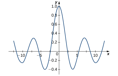
\[y(x)={a}_{0}\sum_{k=0}^{\infty} \frac{{(-1)}^{k}}{{(2)}^{2k}{(k!)}^{2}}{x}^{2k}.\]
The graph appears below for \({a}_{0}=1\) .
Verify that the expression found in Example 2 is a solution to the Bessel equation of order 0.
Key Concepts
- Power series representations of functions can sometimes be used to find solutions to differential equations. (See Example 1.)
- Differentiate the power series term by term and substitute into the differential equation to find relationships between the power series coefficients. (See Example 2.)
Section Exercises
Find a power series solution for the following differential equations.
\({y}^{\prime\prime }+6{y}^{\prime }=0\)
\(5{y}^{\prime\prime }+{y}^{\prime }=0\)
\(y={a}_{0}+5{a}_{1}\sum_{n=1}^{\infty} \frac{{(\text{-}x\text{/}5)}^{n}}{n!}={c}_{0}+5{c}_{1}{e}^{\text{-}x\text{/}5}\)
\({y}^{\prime\prime }+25y=0\)
\({y}^{\prime\prime }-y=0\)
\(y={a}_{0}\sum_{n=0}^{\infty} \frac{{(x)}^{2n}}{(2n)!}+{a}_{1}\sum_{n=0}^{\infty} \frac{{(x)}^{2n+1}}{(2n+1)!}\)
\(2{y}^{\prime }+y=0\)
\({y}^{\prime }-2xy=0\)
\(y={a}_{0}\sum_{n=0}^{\infty} \frac{{x}^{2n}}{n!}={c}_{0}{e}^{{x}^{2}}\)
\((x-7){y}^{\prime }+2y=0\)
\({y}^{\prime\prime }-x{y}^{\prime }-y=0\)
\(y={a}_{0}\sum_{n=0}^{\infty} \frac{{x}^{2n}}{{2}^{n}n!}+{a}_{1}\sum_{n=0}^{\infty} \frac{{x}^{2n+1}}{1\cdot 3\cdot 5\cdot 7\cdots (2n+1)}\)
\((1+{x}^{2}){y}^{\prime\prime }-4x{y}^{\prime }+6y=0\)
\({x}^{2}{y}^{\prime\prime }-x{y}^{\prime }-3y=0\)
\(y={c}_{0}{x}^{3}+\frac{{c}_{1}}{x}\)
\({y}^{\prime\prime }-8{y}^{\prime }=0,\,y(0)=-2,\,\,\,{y}^{\prime }(0)=10\)
\({y}^{\prime\prime }-2xy=0,\,y(0)=1,\,\,\,{y}^{\prime }(0)=-3\)
\(y=1-3x+\frac{2{x}^{3}}{3!}-\frac{12{x}^{4}}{4!}+\frac{16{x}^{6}}{6!}-\frac{120{x}^{7}}{7!}+\cdots\)
The differential equation \({x}^{2}{y}^{\prime\prime }+x{y}^{\prime }+({x}^{2}-1)y=0\) is a Bessel equation of order 1. Use a power series of the form \(y=\sum_{n=0}^{\infty} {a}_{n}{x}^{n}\) to find the solution.
Chapter Review Exercises
True or False? Justify your answer with a proof or a counterexample.
If \(y\) and \(z\) are both solutions to \({y}^{\prime\prime }+2{y}^{\prime }+y=0,\) then \(y+z\) is also a solution.
True
The following system of algebraic equations has a unique solution:
\(\begin{array}{l}6{z}_{1}+3{z}_{2}=8 \\ 4{z}_{1}+2{z}_{2}=4.\end{array}\)
\(y={e}^{x}\text{cos}(3x)+{e}^{x}\text{sin}(2x)\) is a solution to the second-order differential equation \({y}^{\prime\prime }+2y\prime +10=0.\)
False
To find the particular solution to a second-order differential equation, you need one initial condition.
Classify the differential equation. Determine the order, whether it is linear and, if linear, whether the differential equation is homogeneous or nonhomogeneous. If the equation is second-order homogeneous and linear, find the characteristic equation.
\({y}^{\prime\prime }-2y=0\)
second order, linear, homogeneous, \({λ}^{2}-2=0\)
\({y}^{\prime\prime }-3y+2y=\text{cos}\,(t)\)
\({(\frac{dy}{dt})}^{2}+y{y}^{\prime }=1\)
first order, nonlinear, nonhomogeneous
\(\frac{{d}^{2}y}{d{t}^{2}}+t\frac{dy}{dt}+{\text{sin}}^{2}(t)y={e}^{t}\)
For the following problems, find the general solution.
\({y}^{\prime\prime }+9y=0\)
\(y={c}_{1}\text{cos}\,(3x)+{c}_{2}\text{sin}\,(3x)\)
\({y}^{\prime\prime }+2{y}^{\prime }+y=0\)
\({y}^{\prime\prime }-2{y}^{\prime }+10y=4x\)
\(y={c}_{1}{e}^{x}\text{cos}\,(3x)+{c}_{2}{e}^{x}\text{sin}\,(3x)+\frac{2}{5}x+\frac{2}{25}\)
\({y}^{\prime\prime }=\text{cos}\,(x)+2{y}^{\prime }+y\)
\({y}^{''}+5y\prime +4y=x+{e}^{2x}\)
\(y={c}_{1}{e}^{\text{-}x}+{c}_{2}{e}^{-4x}+\frac{x}{4}+\frac{{e}^{2x}}{18}-\frac{5}{16}\)
\({y}^{\prime\prime }=3{y}^{\prime }+x{e}^{\text{-}x}\)
\({y}^{\prime\prime }-{x}^{2}=-3{y}^{\prime }-\frac{9}{4}y+3x\)
\(y={c}_{1}{e}^{(-3\text{/}2)x}+{c}_{2}x{e}^{(-3\text{/}2)x}+\frac{4}{9}{x}^{2}+\frac{4}{27}x-\frac{16}{27}\)
\({y}^{\prime\prime }=2\,\text{cos}\,x+{y}^{\prime }-y\)
For the following problems, find the solution to the initial-value problem, if possible.
\({y}^{\prime\prime }+4{y}^{\prime }+6y=0,\) \(y(0)=0,\) \({y}^{\prime }(0)=\sqrt{2}\)
\(y={e}^{-2x}\text{sin}\,(\sqrt{2}x)\)
\({y}^{\prime\prime }=3y-\text{cos}\,(x),\) \(y(0)=\frac{9}{4},\) \({y}^{\prime }(0)=0\)
For the following problems, find the solution to the boundary-value problem, if possible.
\(4{y}^{\prime }=-6y+2{y}^{\prime\prime },\) \(y(0)=0,\) \(y(1)=1\)
\(y=\frac{{e}^{1-x}}{{e}^{4}-1}({e}^{4x}-1)\)
\({y}^{\prime\prime }=3x-y-{y}^{\prime },\) \(y(0)=-3,\) \(y(1)=0\)
For the following problem, set up and solve the differential equation.
The motion of a swinging pendulum for small angles \(θ\) can be approximated by \(\frac{{d}^{2}θ}{d{t}^{2}}+\frac{g}{L}θ=0,\) where \(θ\) is the angle the pendulum makes with respect to a vertical line, g is the acceleration resulting from gravity, and L is the length of the pendulum. Find the equation describing the angle of the pendulum at time \(t,\) assuming an initial displacement of \({θ}_{0}\) and an initial velocity of zero.
\(θ(t)={θ}_{0}\text{cos}\,(\sqrt{\frac{g}{l}}L)\)
The following problems consider the “beats” that occur when the forcing term of a differential equation causes “slow” and “fast” amplitudes. Consider the general differential equation \(a{y}^{\prime\prime }+by=\text{cos}(ωt)\) that governs undamped motion. Assume that \(\sqrt{\frac{b}{a}}\ne ω\text{.}\)
Find the general solution to this equation (Hint: call \({ω}_{0}=\sqrt{b\text{/}a}\) ).
Assuming the system starts from rest, show that the particular solution can be written as \(y=\frac{2}{a({ω}_{0}{}^{2}-{ω}^{2})}\,\text{sin}\,(\frac{{ω}_{0}-ωt}{2})\,\text{sin}\,(\frac{{ω}_{0}+ωt}{2}).\)
[T] Using your solutions derived earlier, plot the solution to the system \(2{y}^{\prime\prime }+9y=\text{cos}(2t)\) over the interval \(t=[-50,50].\) Find, analytically, the period of the fast and slow amplitudes.
For the following problem, set up and solve the differential equations.
An opera singer is attempting to shatter a glass by singing a particular note. The vibrations of the glass can be modeled by \({y}^{\prime\prime }+ay=0,\) where \(a>0\) represents the natural frequency of the glass and the singer is forcing the vibrations at \(\text{cos}(bt\text{).}\) For what value \(b\) would the singer be able to break that glass? (Note: in order for the glass to break, the oscillations would need to get higher and higher.)
\(b=\sqrt{a}\)