Section 6.8The Divergence Theorem
We have examined several versions of the Fundamental Theorem of Calculus in higher dimensions that relate the integral around an oriented boundary of a domain to a “derivative” of that entity on the oriented domain. In this section, we state the divergence theorem, which is the final theorem of this type that we will study. The divergence theorem has many uses in physics; in particular, the divergence theorem is used in the field of partial differential equations to derive equations modeling heat flow and conservation of mass. We use the theorem to calculate flux integrals and apply it to electrostatic fields.
Overview of Theorems
Before examining the divergence theorem, it is helpful to begin with an overview of the versions of the Fundamental Theorem of Calculus we have discussed:
- The Fundamental Theorem of Calculus:
This theorem relates the integral of derivative \({f}^{\prime }\) over line segment \([a,b]\) along the x-axis to a difference of \(f\) evaluated on the boundary.\[{∫}_{a}^{b}{f}^{\prime }(x)dx=f(b)-f(a).\]
- The Fundamental Theorem for Line Integrals:
where \({P}_{0}\) is the initial point of C and \({P}_{1}\) is the terminal point of C. The Fundamental Theorem for Line Integrals allows path C to be a path in a plane or in space, not just a line segment on the x-axis. If we think of the gradient as a derivative, then this theorem relates an integral of derivative \(∇f\) over path C to a difference of \(f\) evaluated on the boundary of C.\[{∫}_{C}∇f·d\text{r}=f({P}_{1})-f({P}_{0}),\]
- Green’s theorem, circulation form:
Since \({Q}_{x}-{P}_{y}=\text{curl}\,\text{F}·\text{k}\) and curl is a derivative of sorts, Green’s theorem relates the integral of derivative curlF over planar region D to an integral of F over the boundary of D.\[{∬}_{D}({Q}_{x}-{P}_{y})dA={∫}_{C}\text{F}·d\text{r}.\]
- Green’s theorem, flux form:
Since \({P}_{x}+{Q}_{y}=\text{div}\,\text{F}\) and divergence is a derivative of sorts, the flux form of Green’s theorem relates the integral of derivative divF over planar region D to an integral of F over the boundary of D.\[{∬}_{D}({P}_{x}+{Q}_{y})dA={∫}_{C}\text{F}·\text{N}ds.\]
- Stokes’ theorem:
If we think of the curl as a derivative of sorts, then Stokes’ theorem relates the integral of derivative curlF over surface S (not necessarily planar) to an integral of F over the boundary of S.\[{∬}_{S}\text{curl}\,\text{F}·d\text{S}={∫}_{C}\text{F}·d\text{r}.\]
Stating the Divergence Theorem
The divergence theorem follows the general pattern of these other theorems. If we think of divergence as a derivative of sorts, then the divergence theorem relates a triple integral of derivative divF over a solid to a flux integral of F over the boundary of the solid. More specifically, the divergence theorem relates a flux integral of vector field F over a closed surface S to a triple integral of the divergence of F over the solid enclosed by S.
Let S be a piecewise, smooth closed surface that encloses solid E in space. Assume that S is oriented outward, and let F be a vector field with continuous partial derivatives on an open region containing E (Figure 1). Then
\[{∭}_{E}\text{div}\,\text{F}dV=\underset{S}{∬}\text{F}·d\text{S}.\]
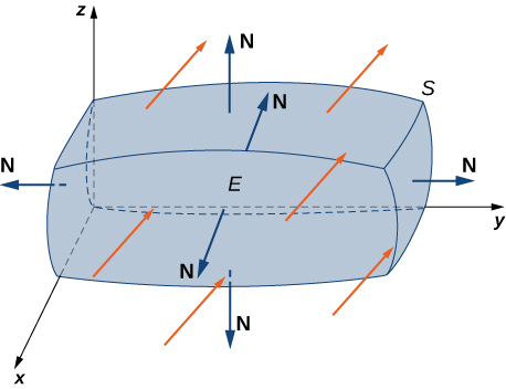
Recall that the flux form of Green’s theorem states that \({∬}_{D}\text{div}\,\text{F}dA={∫}_{C}\text{F}·\text{N}ds.\) Therefore, the divergence theorem is a version of Green’s theorem in one higher dimension.
The proof of the divergence theorem is beyond the scope of this text. However, we look at an informal proof that gives a general feel for why the theorem is true, but does not prove the theorem with full rigor. This explanation follows the informal explanation given for why Stokes’ theorem is true.
Proof
Let B be a small box with sides parallel to the coordinate planes inside E (Figure 2). Let the center of B have coordinates \((x,y,z)\) and suppose the edge lengths are \(\Delta x,\Delta y,\) and \(\Delta z\) (Figure 2(b)). The normal vector out of the top of the box is k and the normal vector out of the bottom of the box is \(\text{-}\text{k}.\) The dot product of \(\text{F}=\langle P,Q,R\rangle\) with k is R and the dot product with \(\text{-}\text{k}\) is \(\text{-}R.\) The area of the top of the box (and the bottom of the box) \(\Delta S\) is \(\Delta x\Delta y.\)
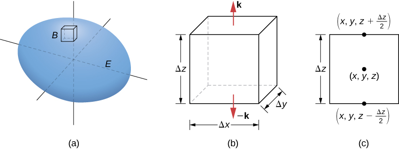
The flux out of the top of the box can be approximated by \(R(x,y,z+\frac{\Delta z}{2})\Delta x\Delta y\) (Figure 2(c)) and the flux out of the bottom of the box is \(\text{-}R(x,y,z-\frac{\Delta z}{2})\Delta x\Delta y.\) If we denote the difference between these values as \(\Delta R,\) then the net flux in the vertical direction can be approximated by \(\Delta R\Delta x\Delta y.\) However,
\[\Delta R\Delta x\Delta y=(\frac{\Delta R}{\Delta z})\Delta x\Delta y\Delta z\approx (\frac{∂R}{∂z})\Delta V.\]
Therefore, the net flux in the vertical direction can be approximated by \((\frac{∂R}{∂z})\Delta V.\) Similarly, the net flux in the x-direction can be approximated by \((\frac{∂P}{∂x})\Delta V\) and the net flux in the y-direction can be approximated by \((\frac{∂Q}{∂y})\Delta V.\) Adding the fluxes in all three directions gives an approximation of the total flux out of the box:
\[\text{Total flux}\approx (\frac{∂P}{∂x}+\frac{∂Q}{∂y}+\frac{∂R}{∂z})\Delta V=\text{div}\,\text{F}\Delta V.\]
This approximation becomes arbitrarily close to the value of the total flux as the volume of the box shrinks to zero.
The sum of \(\text{div}\,\text{F}\Delta V\) over all the small boxes approximating E is approximately \({∭}_{E}\text{div}\,\text{F}dV.\) On the other hand, the sum of \(\text{div}\,\text{F}\Delta V\) over all the small boxes approximating E is the sum of the fluxes over all these boxes. Just as in the informal proof of Stokes’ theorem, adding these fluxes over all the boxes results in the cancelation of a lot of the terms. If an approximating box shares a face with another approximating box, then the flux over one face is the negative of the flux over the shared face of the adjacent box. These two integrals cancel out. When adding up all the fluxes, the only flux integrals that survive are the integrals over the faces approximating the boundary of E. As the volumes of the approximating boxes shrink to zero, this approximation becomes arbitrarily close to the flux over S.
□
Verify the divergence theorem for vector field \(\text{F}=\langle x-y,x+z,z-y\rangle\) and surface S that consists of cone \({x}^{2}+{y}^{2}={z}^{2},0\le z\le 1,\) and the circular top of the cone (see the following figure). Assume this surface is oriented outward.
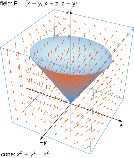
Compute both sides separately: the triple integral of div F over the solid cone, and the flux of F over the two pieces of the boundary (the slanted side and the circular top).
Let E be the solid cone enclosed by S. To verify the theorem for this example, we show that \({∭}_{E}\text{div}\,\text{F}dV=\underset{S}{∬}\text{F}·d\text{S}\) by calculating each integral separately.
To compute the triple integral, note that \(\text{div}\,\text{F}={P}_{x}+{Q}_{y}+{R}_{z}=2,\) and therefore the triple integral is
\[\begin{array}{ll}{∭}_{E}\text{div}\,\text{F}dV & =2{∭}_{E}dV \\ & =2(\text{volume of}\,E).\end{array}\]
The volume of a right circular cone is given by \(\pi {r}^{2}\frac{h}{3}.\) In this case, \(h=r=1.\) Therefore,
\[{∭}_{E}\text{div}\,\text{F}dV=2(\text{volume of}\,E)=\frac{2\pi }{3}.\]
To compute the flux integral, first note that S is piecewise smooth; S can be written as a union of smooth surfaces. Therefore, we break the flux integral into two pieces: one flux integral across the circular top of the cone and one flux integral across the remaining portion of the cone. Call the circular top \({S}_{1}\) and the portion under the top \({S}_{2}.\) We start by calculating the flux across the circular top of the cone. Notice that \({S}_{1}\) has parameterization
\[\text{r}(u,v)=\langle u\,\text{cos}\,v,u\,\text{sin}\,v,1\rangle ,0\le u\le 1,0\le v\le 2\pi .\]
Then, the tangent vectors are \({\text{t}}_{u}=\langle \text{cos}\,v,\text{sin}\,v,0\rangle\) and \({\text{t}}_{v}=\langle \text{-}u\,\text{cos}\,v,u\,\text{sin}\,v,0\rangle .\) Therefore, the flux across \({S}_{1}\) is
\[\begin{array}{ll}{∬}_{{S}_{1}}\text{F}·d\text{S} & ={∫}_{0}^{1}{∫}_{0}^{2\pi }\text{F}(\text{r}(u,v))·({\text{t}}_{u}\,\times \,{\text{t}}_{v})dA \\ & ={∫}_{0}^{1}{∫}_{0}^{2\pi }\langle u\,\text{cos}\,v-u\,\text{sin}\,v,u\,\text{cos}\,v+1,1-u\,\text{sin}\,v\rangle ·\langle 0,0,u\rangle dvdu \\ & ={∫}_{0}^{1}{∫}_{0}^{2\pi }u-{u}^{2}\text{sin}\,v\,dvdu=\pi .\end{array}\]
We now calculate the flux over \({S}_{2}.\) A parameterization of this surface is
\[\text{r}(u,v)=\langle u\,\text{cos}\,v,u\,\text{sin}\,v,u\rangle ,0\le u\le 1,0\le v\le 2\pi .\]
The tangent vectors are \({\text{t}}_{u}=\langle \text{cos}\,v,\text{sin}\,v,1\rangle\) and \({\text{t}}_{v}=\langle \text{-}u\,\text{sin}\,v,u\,\text{cos}\,v,0\rangle ,\) so the cross product is
\[{\text{t}}_{u}\,\times \,{\text{t}}_{v}=\langle \text{-}u\,\text{cos}\,v,\text{-}u\,\text{sin}\,v,u\rangle .\]
Notice that the negative signs on the x and y components induce the inward orientation of the cone. Since the surface is oriented outward, we use vector \({\text{t}}_{v}\,\times \,{\text{t}}_{u}=\langle u\,\text{cos}\,v,u\,\text{sin}\,v,\text{-}u\rangle\) in the flux integral. The flux across \({S}_{2}\) is then
\[\begin{array}{ll}{∬}_{{S}_{2}}\text{F}·d\text{S} & ={∫}_{0}^{1}{∫}_{0}^{2\pi }\text{F}(\text{r}(u,v))·({\text{t}}_{v}\,\times \,{\text{t}}_{u})dA \\ & ={∫}_{0}^{1}{∫}_{0}^{2\pi }\langle u\,\text{cos}\,v-u\,\text{sin}\,v,u\,\text{cos}\,v+u,u-\text{sin}\,v\rangle ·\langle u\,\text{cos}\,v,u\,\text{sin}\,v,\text{-}u\rangle \\ & ={∫}_{0}^{1}{∫}_{0}^{2\pi }{u}^{2}{\text{cos}}^{2}v+2{u}^{2}\text{sin}\,v-{u}^{2}dvdu=-\frac{\pi }{3}.\end{array}\]
The total flux across S is
\[{∬}_{{S}_{2}}\text{F}·d\text{S}={∬}_{{S}_{1}}\text{F}·d\text{S}+{∬}_{{S}_{2}}\text{F}·d\text{S}=\frac{2\pi }{3}={∭}_{E}\text{div}\,\text{F}dV,\]
and we have verified the divergence theorem for this example.
Verify the divergence theorem for vector field \(\text{F}(x,y,z)=\langle x+y+z,y,2x-y\rangle\) and surface S given by the cylinder \({x}^{2}+{y}^{2}=1,0\le z\le 3\) plus the circular top and bottom of the cylinder. Assume that S is oriented outward.
Both integrals equal \(6\pi .\)
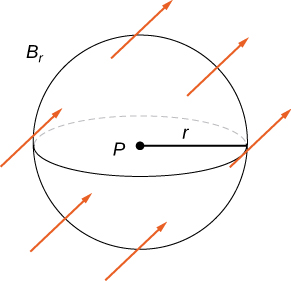
Recall that the divergence of continuous field F at point P is a measure of the “outflowing-ness” of the field at P. If F represents the velocity field of a fluid, then the divergence can be thought of as the rate per unit volume of the fluid flowing out less the rate per unit volume flowing in. The divergence theorem confirms this interpretation. To see this, let P be a point and let \({B}_{r}\) be a ball of small radius r centered at P (Figure 3). Let \({S}_{r}\) be the boundary sphere of \({B}_{r}.\) Since the radius is small and F is continuous, \(\text{div}\,\text{F}(Q)\approx \text{div}\,\text{F}(P)\) for all other points Q in the ball. Therefore, the flux across \({S}_{r}\) can be approximated using the divergence theorem:
\[{∬}_{{S}_{r}}\text{F}·d\text{S}={∭}_{{B}_{r}}\text{div}\,\text{F}dV\approx {∭}_{{B}_{r}}\text{div}\,\text{F}(P)dV.\]
Since \(\text{div}\,\text{F}(P)\) is a constant,
\[{∭}_{{B}_{r}}\text{div}\,\text{F}(P)dV=\text{div}\,\text{F}(P)V({B}_{r}).\]
Therefore, flux \({∬}_{{S}_{r}}\text{F}·d\text{S}\) can be approximated by \(\text{div}\,\text{F}(P)V({B}_{r}).\) This approximation gets better as the radius shrinks to zero, and therefore
\[\text{div}\,\text{F}(P)=\underset{r\to 0}{\text{lim}}\frac{1}{V({B}_{r})}{∬}_{{S}_{r}}\text{F}·d\text{S}.\]
This equation says that the divergence at P is the net rate of outward flux of the fluid per unit volume.
Using the Divergence Theorem
The divergence theorem translates between the flux integral of closed surface S and a triple integral over the solid enclosed by S. Therefore, the theorem allows us to compute flux integrals or triple integrals that would ordinarily be difficult to compute by translating the flux integral into a triple integral and vice versa.
Calculate the surface integral \({∬}_{S}\text{F}·d\text{S},\) where S is cylinder \({x}^{2}+{y}^{2}=1,0\le z\le 2,\) including the circular top and bottom, and \(\text{F}=\langle \frac{{x}^{3}}{3}+yz,\frac{{y}^{3}}{3}-\text{sin}(xz),z-x-y\rangle .\)
Rather than parameterizing all three pieces of the boundary, compute div F and convert the flux integral into a triple integral in cylindrical coordinates.
We could calculate this integral without the divergence theorem, but the calculation is not straightforward because we would have to break the flux integral into three separate integrals: one for the top of the cylinder, one for the bottom, and one for the side. Furthermore, each integral would require parameterizing the corresponding surface, calculating tangent vectors and their cross product, and using (see original).
By contrast, the divergence theorem allows us to calculate the single triple integral \({∭}_{E}\text{div}\,\text{F}dV,\) where E is the solid enclosed by the cylinder. Using the divergence theorem and converting to cylindrical coordinates, we have
\[\begin{array}{ll}{∬}_{s}\text{F}·d\text{S} & ={∭}_{E}\text{div}\,\text{F}\,dV \\ & ={∭}_{E}({x}^{2}+{y}^{2}+1)dV \\ & ={∫}_{0}^{2\pi }{∫}_{0}^{1}{∫}_{0}^{2}({r}^{2}+1)r\,dz\,dr\,dθ \\ & =\frac{3}{2}{∫}_{0}^{2\pi }dθ=3\pi .\end{array}\]
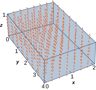
Use the divergence theorem to calculate flux integral \({∬}_{S}\text{F}·d\text{S},\) where S is the boundary of the box given by \(0\le x\le 2,1\le y\le 4,0\le z\le 1,\) and \(\text{F}=\langle {x}^{2}+yz,y-z,2x+2y+2z\rangle\) (see the following figure).
30
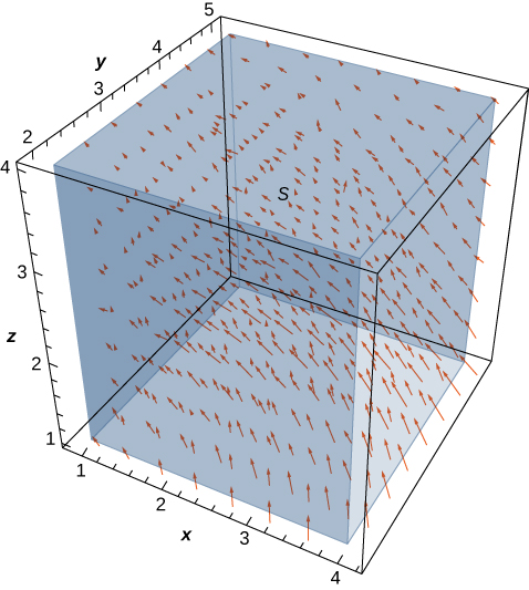
Let \(\text{v}=\langle -\frac{y}{z},\frac{x}{z},0\rangle\) be the velocity field of a fluid. Let C be the solid cube given by \(1\le x\le 4,2\le y\le 5,1\le z\le 4,\) and let S be the boundary of this cube (see the following figure). Find the flow rate of the fluid across S.
Compute div v first — if it comes out to zero, the divergence theorem immediately tells you the flux integral is zero, without any surface work.
The flow rate of the fluid across S is \({∬}_{S}\text{v}·d\text{S}.\) Before calculating this flux integral, let’s discuss what the value of the integral should be. Based on Figure 4, we see that if we place this cube in the fluid (as long as the cube doesn’t encompass the origin), then the rate of fluid entering the cube is the same as the rate of fluid exiting the cube. The field is rotational in nature and, for a given circle parallel to the xy-plane that has a center on the z-axis, the vectors along that circle are all the same magnitude. That is how we can see that the flow rate is the same entering and exiting the cube. The flow into the cube cancels with the flow out of the cube, and therefore the flow rate of the fluid across the cube should be zero.
To verify this intuition, we need to calculate the flux integral. Calculating the flux integral directly requires breaking the flux integral into six separate flux integrals, one for each face of the cube. We also need to find tangent vectors, compute their cross product, and use (see original). However, using the divergence theorem makes this calculation go much more quickly:
\[\begin{array}{ll}{∬}_{S}\text{v}·d\text{S} & ={∭}_{C}\text{div}(\text{v})dV \\ & ={∭}_{C}0\,dV=0.\end{array}\]
Therefore the flux is zero, as expected.
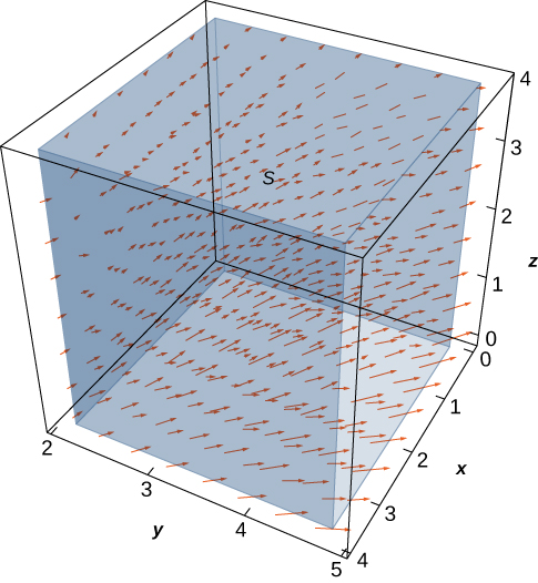
Let \(\text{v}=\langle \frac{x}{z},\frac{y}{z},0\rangle\) be the velocity field of a fluid. Let C be the solid cube given by \(1\le x\le 4,2\le y\le 5,1\le z\le 4,\) and let S be the boundary of this cube (see the following figure). Find the flow rate of the fluid across S.
\(9\,\text{ln}(16)\)
Example 3 illustrates a remarkable consequence of the divergence theorem. Let S be a piecewise, smooth closed surface and let F be a vector field defined on an open region containing the surface enclosed by S. If F has the form \(\text{F}=\langle f(y,z),g(x,z),h(x,y)\rangle ,\) then the divergence of F is zero. By the divergence theorem, the flux of F across S is also zero. This makes certain flux integrals incredibly easy to calculate. For example, suppose we wanted to calculate the flux integral \({∬}_{S}\text{F}·d\text{S}\) where S is a cube and
\[\text{F}=\langle \text{sin}(y){e}^{yz},{x}^{2}{z}^{2},\text{cos}(xy){e}^{\text{sin}\,x}\rangle .\]
Calculating the flux integral directly would be difficult, if not impossible, using techniques we studied previously. At the very least, we would have to break the flux integral into six integrals, one for each face of the cube. But, because the divergence of this field is zero, the divergence theorem immediately shows that the flux integral is zero.
We can now use the divergence theorem to justify the physical interpretation of divergence that we discussed earlier. Recall that if F is a continuous three-dimensional vector field and P is a point in the domain of F, then the divergence of F at P is a measure of the “outflowing-ness” of F at P. If F represents the velocity field of a fluid, then the divergence of F at P is a measure of the net flow rate out of point P (the flow of fluid out of P less the flow of fluid in to P). To see how the divergence theorem justifies this interpretation, let \({B}_{r}\) be a ball of very small radius r with center P, and assume that \({B}_{r}\) is in the domain of F. Furthermore, assume that \({B}_{r}\) has a positive, outward orientation. Since the radius of \({B}_{r}\) is small and F is continuous, the divergence of F is approximately constant on \({B}_{r}.\) That is, if \({P}^{\prime }\) is any point in \({B}_{r},\) then \(\text{div}\,\text{F}(P)\approx \text{div}\,\text{F}({P}^{\prime }).\) Let \({S}_{r}\) denote the boundary sphere of \({B}_{r}.\) We can approximate the flux across \({S}_{r}\) using the divergence theorem as follows:
\[\begin{array}{ll}{∬}_{{S}_{r}}\text{F}·d\text{S} & ={∭}_{{B}_{r}}\text{div}\,\text{F}\,dV \\ & \approx {∭}_{{B}_{r}}\text{div}\,\text{F}(P)dV \\ & =\text{div}\,\text{F}(P)V({B}_{r}).\end{array}\]
As we shrink the radius r to zero via a limit, the quantity \(\text{div}\,\text{F}(P)V({B}_{r})\) gets arbitrarily close to the flux. Therefore,
\[\text{div}\,\text{F}(P)=\underset{r\to 0}{\text{lim}}\frac{1}{V({B}_{r})}{∬}_{{S}_{r}}\text{F}·d\text{S}\]
and we can consider the divergence at P as measuring the net rate of outward flux per unit volume at P. Since “outflowing-ness” is an informal term for the net rate of outward flux per unit volume, we have justified the physical interpretation of divergence we discussed earlier, and we have used the divergence theorem to give this justification.
Application to Electrostatic Fields
The divergence theorem has many applications in physics and engineering. It allows us to write many physical laws in both an integral form and a differential form (in much the same way that Stokes’ theorem allowed us to translate between an integral and differential form of Faraday’s law). Areas of study such as fluid dynamics, electromagnetism, and quantum mechanics have equations that describe the conservation of mass, momentum, or energy, and the divergence theorem allows us to give these equations in both integral and differential forms.
One of the most common applications of the divergence theorem is to electrostatic fields. An important result in this subject is Gauss’ law. This law states that if S is a closed surface in electrostatic field E, then the flux of E across S is the total charge enclosed by S (divided by an electric constant). We now use the divergence theorem to justify the special case of this law in which the electrostatic field is generated by a stationary point charge at the origin.
If \((x,y,z)\) is a point in space, then the distance from the point to the origin is \(r=\sqrt{{x}^{2}+{y}^{2}+{z}^{2}}.\) Let \({\text{F}}_{r}\) denote radial vector field \({\text{F}}_{r}=\frac{1}{{r}^{2}}\langle \frac{x}{r},\frac{y}{r},\frac{z}{r}\rangle .\) The vector at a given position in space points in the direction of unit radial vector \(\langle \frac{x}{r},\frac{y}{r},\frac{z}{r}\rangle\) and is scaled by the quantity \(1\text{/}{r}^{2}.\) Therefore, the magnitude of a vector at a given point is inversely proportional to the square of the vector’s distance from the origin. Suppose we have a stationary charge of q Coulombs at the origin, existing in a vacuum. The charge generates electrostatic field E given by
\[\text{E}=\frac{q}{4\pi {ε}_{0}}{\text{F}}_{r},\]
where the approximation \({ε}_{0}=8.854\,\times \,{10}^{-12}\) farad (F)/m is an electric constant. (The constant \({ε}_{0}\) is a measure of the resistance encountered when forming an electric field in a vacuum.) Notice that E is a radial vector field similar to the gravitational field described in (see original). The difference is that this field points outward whereas the gravitational field points inward. Because
\[\text{E}=\frac{q}{4\pi {ε}_{0}}{\text{F}}_{r}=\frac{q}{4\pi {ε}_{0}}(\frac{1}{{r}^{2}}\langle \frac{x}{r},\frac{y}{r},\frac{z}{r}\rangle ),\]
we say that electrostatic fields obey an inverse-square law. That is, the electrostatic force at a given point is inversely proportional to the square of the distance from the source of the charge (which in this case is at the origin). Given this vector field, we show that the flux across closed surface S is zero if the charge is outside of S, and that the flux is \(q\text{/}{ε}_{0}\) if the charge is inside of S. In other words, the flux across S is the charge inside the surface divided by constant \({ε}_{0}.\) This is a special case of Gauss’ law, and here we use the divergence theorem to justify this special case.
To show that the flux across S is the charge inside the surface divided by constant \({ε}_{0},\) we need two intermediate steps. First we show that the divergence of \({\text{F}}_{r}\) is zero and then we show that the flux of \({\text{F}}_{r}\) across any smooth surface S is either zero or \(4\pi .\) We can then justify this special case of Gauss’ law.
Verify that the divergence of \({\text{F}}_{r}\) is zero where \({\text{F}}_{r}\) is defined (away from the origin).
Use the quotient rule to compute \(\partial/\partial x(x/r^3)\), then find the analogous y and z partials and add them.
Since \(r=\sqrt{{x}^{2}+{y}^{2}+{z}^{2}},\) the quotient rule gives us
\[\begin{array}{ll}\frac{∂}{∂x}(\frac{x}{{r}^{3}}) & =\frac{∂}{∂x}(\frac{x}{{({x}^{2}+{y}^{2}+{z}^{2})}^{3\text{/}2}}) \\ & =\frac{{({x}^{2}+{y}^{2}+{z}^{2})}^{3\text{/}2}-x[\frac{3}{2}{({x}^{2}+{y}^{2}+{z}^{2})}^{1\text{/}2}2x]}{{({x}^{2}+{y}^{2}+{z}^{2})}^{3}} \\ & =\frac{{r}^{3}-3{x}^{2}r}{{r}^{6}}=\frac{{r}^{2}-3{x}^{2}}{{r}^{5}}.\end{array}\]
Similarly,
\[\frac{∂}{∂y}(\frac{y}{{r}^{3}})=\frac{{r}^{2}-3{y}^{2}}{{r}^{5}}\,\text{and}\,\frac{∂}{∂z}(\frac{z}{{r}^{3}})=\frac{{r}^{2}-3{z}^{2}}{{r}^{5}}.\]
Therefore,
\[\begin{array}{ll}\text{div}\,{\text{F}}_{r} & =\frac{{r}^{2}-3{x}^{2}}{{r}^{5}}+\frac{{r}^{2}-3{y}^{2}}{{r}^{5}}+\frac{{r}^{2}-3{z}^{2}}{{r}^{5}} \\ & =\frac{3{r}^{2}-3({x}^{2}+{y}^{2}+{z}^{2})}{{r}^{5}} \\ & =\frac{3{r}^{2}-3{r}^{2}}{{r}^{5}}=0.\end{array}\]
Notice that since the divergence of \({\text{F}}_{r}\) is zero and E is \({\text{F}}_{r}\) scaled by a constant, the divergence of electrostatic field E is also zero (except at the origin).
Let S be a connected, piecewise smooth closed surface and let \({\text{F}}_{r}=\frac{1}{{r}^{2}}\langle \frac{x}{r},\frac{y}{r},\frac{z}{r}\rangle .\) Then,
\[{∬}_{S}{\text{F}}_{r}·d\text{S}=\left\{\begin{array}{llll}0 & & & \text{if}\,S\,\text{does not encompass the origin} \\ 4\pi & & & \text{if}\,S\,\text{encompasses the origin.}\end{array}\right.\]
In other words, this theorem says that the flux of \({\text{F}}_{r}\) across any piecewise smooth closed surface S depends only on whether the origin is inside of S.
Proof
The logic of this proof follows the logic of (see original), only we use the divergence theorem rather than Green’s theorem.
First, suppose that S does not encompass the origin. In this case, the solid enclosed by S is in the domain of \({\text{F}}_{r},\) and since the divergence of \({\text{F}}_{r}\) is zero, we can immediately apply the divergence theorem and find that \({∬}_{S}\text{F}·d\text{S}\) is zero.
Now suppose that S does encompass the origin. We cannot just use the divergence theorem to calculate the flux, because the field is not defined at the origin. Let \({S}_{a}\) be a sphere of radius a inside of S centered at the origin. The outward normal vector field on the sphere, in spherical coordinates, is
\[{\text{t}}_{ϕ}\,\times \,{\text{t}}_{θ}=\langle {a}^{2}\text{cos}\,θ\,{\text{sin}}^{2}ϕ,{a}^{2}\text{sin}\,θ\,{\text{sin}}^{2}ϕ,{a}^{2}\text{sin}\,ϕ\,\text{cos}\,ϕ\rangle \]
(see (see original)). Therefore, on the surface of the sphere, the dot product \({\text{F}}_{r}·\text{N}\) (in spherical coordinates) is
\[\begin{array}{ll}{\text{F}}_{r}·\text{N} & =\langle \frac{\text{sin}\,ϕ\,\text{cos}\,θ}{{a}^{2}},\frac{\text{sin}\,ϕ\,\text{sin}\,θ}{{a}^{2}},\frac{\text{cos}\,ϕ}{{a}^{2}}\rangle ·\langle {a}^{2}\text{cos}\,θ\,{\text{sin}}^{2}ϕ,{a}^{2}\text{sin}\,θ\,{\text{sin}}^{2}ϕ,{a}^{2}\text{sin}\,ϕ\,\text{cos}\,ϕ\rangle \\ & =\text{sin}\,ϕ(\langle \text{sin}\,ϕ\,\text{cos}\,θ,\text{sin}\,ϕ\,\text{sin}\,θ,\text{cos}\,ϕ\rangle ·\langle \text{sin}\,ϕ\,\text{cos}\,θ,\text{sin}\,ϕ\,\text{sin}\,θ,\text{cos}\,ϕ\rangle ) \\ & =\text{sin}\,ϕ.\end{array}\]
The flux of \({\text{F}}_{r}\) across \({S}_{a}\) is
\[{∬}_{{S}_{a}}{\text{F}}_{r}·\text{N}dS={∫}_{0}^{2\pi }{∫}_{0}^{\pi }\text{sin}\,ϕdϕdθ=4\pi .\]
Now, remember that we are interested in the flux across S, not necessarily the flux across \({S}_{a}.\) To calculate the flux across S, let E be the solid between surfaces \({S}_{a}\) and S. Then, the boundary of E consists of \({S}_{a}\) and S. Denote this boundary by \(S-{S}_{a}\) to indicate that S is oriented outward but now \({S}_{a}\) is oriented inward. We would like to apply the divergence theorem to solid E. Notice that the divergence theorem, as stated, can’t handle a solid such as E because E has a hole. However, the divergence theorem can be extended to handle solids with holes, just as Green’s theorem can be extended to handle regions with holes. This allows us to use the divergence theorem in the following way. By the divergence theorem,
\[\begin{array}{ll}{∬}_{S-{S}_{a}}{\text{F}}_{r}·d\text{S} & ={∬}_{S}{\text{F}}_{r}·d\text{S}-{∬}_{{S}_{a}}{\text{F}}_{r}·d\text{S} \\ & ={∭}_{E}\text{div}{\text{F}}_{r}\,dV \\ & ={∭}_{E}0dV=0.\end{array}\]
Therefore,
\[{∬}_{S}{\text{F}}_{r}·d\text{S}={∬}_{{S}_{a}}{\text{F}}_{r}·d\text{S}=4\pi ,\]
and we have our desired result.
□
Now we return to calculating the flux across a smooth surface in the context of electrostatic field \(\text{E}=\frac{q}{4\pi {ε}_{0}}{\text{F}}_{r}\) of a point charge at the origin. Let S be a piecewise smooth closed surface that encompasses the origin. Then
\[\begin{array}{ll}{∬}_{S}\text{E}·d\text{S} & ={∬}_{S}\frac{q}{4\pi {ε}_{0}}{\text{F}}_{r}·d\text{S} \\ & =\frac{q}{4\pi {ε}_{0}}{∬}_{S}{\text{F}}_{r}·d\text{S} \\ & =\frac{q}{{ε}_{0}}.\end{array}\]
If S does not encompass the origin, then
\[{∬}_{S}\text{E}·d\text{S}=\frac{q}{4\pi {ε}_{0}}{∬}_{S}{\text{F}}_{r}·d\text{S}=0.\]
Therefore, we have justified the claim that we set out to justify: the flux across closed surface S is zero if the charge is outside of S, and the flux is \(q\text{/}{ε}_{0}\) if the charge is inside of S.
This analysis works only if there is a single point charge at the origin. In this case, Gauss’ law says that the flux of E across S is the total charge enclosed by S. Gauss’ law can be extended to handle multiple charged solids in space, not just a single point charge at the origin. The logic is similar to the previous analysis, but beyond the scope of this text. In full generality, Gauss’ law states that if S is a piecewise smooth closed surface and Q is the total amount of charge inside of S, then the flux of E across S is \(Q\text{/}{ε}_{0}.\)
Suppose we have four stationary point charges in space, all with a charge of 0.002 Coulombs (C). The charges are located at \((0,1,1),(1,1,4),(-1,0,0),\,\text{and}\,(-2,-2,2).\) Let E denote the electrostatic field generated by these point charges. If S is the sphere of radius 2 oriented outward and centered at the origin, then find \({∬}_{S}\text{E}·d\text{S}.\)
Check which of the four charges actually lie inside the radius-2 sphere, sum only those, then apply Gauss's law.
According to Gauss’ law, the flux of E across S is the total charge inside of S divided by the electric constant. Since S has radius 2, notice that only two of the charges are inside of S: the charge at \((0,1,1)\) and the charge at \((-1,0,0).\) Therefore, the total charge encompassed by S is 0.004 and, by Gauss’ law,
\[{∬}_{S}\text{E}·d\text{S}=\frac{0.004}{8.854\,\times \,{10}^{-12}}\approx 4.518\,\times \,{10}^{9}\,\text{V-m}.\]
Work the previous example for surface S that is a sphere of radius 4 centered at the origin, oriented outward.
\(\approx 6.777\,\times \,{10}^{9}\)
Key Concepts
- The divergence theorem relates a surface integral across closed surface S to a triple integral over the solid enclosed by S. The divergence theorem is a higher dimensional version of the flux form of Green’s theorem, and is therefore a higher dimensional version of the Fundamental Theorem of Calculus. (See Example 1.)
- The divergence theorem can be used to transform a difficult flux integral into an easier triple integral and vice versa. (See Example 2 and Example 3.)
- The divergence theorem can be used to derive Gauss’ law, a fundamental law in electrostatics. (See Example 4 and Example 5.)
Key Equations
| Divergence theorem | \({∭}_{E}\text{div}\,\text{F}dV=\underset{S}{∬}\text{F}·d\text{S}\) |
Section Exercises
For the following exercises, use a computer algebraic system (CAS) and the divergence theorem to evaluate surface integral \({∬}_{S}^{}\text{F}·\text{N}ds\) for the given choice of F and the boundary surface S. For each closed surface, assume N is the outward unit normal vector.
[T] \(\text{F}(x,y,z)=x\text{i}+y\text{j}+z\text{k};\) S is the surface of cube \(0\le x\le 1,0\le y\le 1,0<z\le 1.\)
[T] \(\text{F}(x,y,z)=(\text{cos}\,yz)\text{i}+{e}^{xz}\text{j}+3{z}^{2}\text{k}\text{;}\) S is the surface of hemisphere \(z=\sqrt{4-{x}^{2}-{y}^{2}}\) together with disk \({x}^{2}+{y}^{2}\le 4\) in the xy-plane.
\({∫}_{S}^{}\text{F}·\text{N}ds=24\pi \approx 75.3982\)
[T] \(\text{F}(x,y,z)=({x}^{2}+{y}^{2}-{x}^{2})\text{i}+{x}^{2}y\text{j}+3z\text{k};S\) is the surface of the unit cube \(0\le x\le 1,0\le y\le 1,0\le z\le 1\) excluding the face \(z=0\) .
[T] \(\text{F}(x,y,z)=x\text{i}+y\text{j}+z\text{k}\text{;}\) S is the surface of the solid bounded by the parabola \(z={x}^{2}+{y}^{2}\,\) and the plane \(z=9\) .
\({∫}_{S}^{}\text{F}·\text{N}ds=\frac{243\pi }{2}\approx 381.704\)
[T] \(\text{F}(x,y,z)={x}^{2}\text{i}+{y}^{2}\text{j}+{z}^{2}\text{k}\text{;}\) S is the surface of sphere \({x}^{2}+{y}^{2}+{z}^{2}=4.\)
[T] \(\text{F}(x,y,z)=x\text{i}+y\text{j}+({z}^{2}-1)\text{k}\text{;}\) S is the surface of the solid bounded by cylinder \({x}^{2}+{y}^{2}=4\) and planes \(z=0\,\text{and}\,z=1.\)
\({∫}_{S}^{}\text{F}·\text{N}ds=12\pi \approx 37.6991\)
[T] \(\text{F}(x,y,z)=x{y}^{2}\text{i}+y{z}^{2}\text{j}+{x}^{2}z\text{k}\text{;}\) S is the surface of the solid bounded above by sphere \(ρ=2\) and below by cone \(φ=\frac{\pi }{4}\) in spherical coordinates. (Think of S as the surface of an “ice cream cone.”)
[T] \(\text{F}(x,y,z)={x}^{3}\text{i}+{y}^{3}\text{j}+3{a}^{2}z\text{k}\,\text{(constant}\,a>0)\text{;}\) S is the surface of the solid bounded by cylinder \({x}^{2}+{y}^{2}={a}^{2}\) and planes \(z=0\,\text{and}\,z=1.\)
\({∫}_{S}^{}\text{F}·\text{N}ds=\frac{9\pi {a}^{4}}{2}\)
[T] Surface integral \({∬}_{S}\text{F}·d\text{S},\) where S is the surface of the solid bounded by paraboloid \(z={x}^{2}+{y}^{2}\) and plane \(z=4,\) and \(\text{F}(x,y,z)=(x+{y}^{2}{z}^{2})\text{i}+(y+{z}^{2}{x}^{2})\text{j}+(z+{x}^{2}{y}^{2})\text{k}\)
Use the divergence theorem to calculate surface integral \({∬}_{S}\text{F}·d\text{S},\) where \(\text{F}(x,y,z)=({e}^{{y}^{2}})\text{i}+(y+\text{sin}({z}^{2}))\text{j}+(z-1)\text{k}\) and S is the surface of the solid bounded by the sphere \({x}^{2}+{y}^{2}+{z}^{2}=1\text{,}\) and below by the plane \(z=0\) .
\({∬}_{S}\text{F}·d\text{S}=\frac{4\pi }{3}\)
Use the divergence theorem to calculate surface integral \({∬}_{S}\text{F}·ds,\) where \(\text{F}(x,y,z)={x}^{4}\text{i}-{x}^{3}{z}^{2}\text{j}+4x{y}^{2}z\text{k}\) and \(S\) is the surface bounded by cylinder \({x}^{2}+{y}^{2}=1\) and planes \(z=x+2\) and \(z=0.\)
Use the divergence theorem to calculate surface integral \({∬}_{S}\text{F}·d\text{S}\) when \(\text{F}(x,y,z)={x}^{2}{z}^{3}\text{i}+2xy{z}^{3}\text{j}+x{z}^{4}\text{k}\) and S is the surface of the box with vertices \((\pm 1,\pm 2,\pm 3).\)
\({∬}_{S}\text{F}·d\text{S}=0\)
Use the divergence theorem to calculate surface integral \({∬}_{S}\text{F}·d\text{S}\) when \(\text{F}(x,y,z)=z\,{\text{tan}}^{-1}({y}^{2})\text{i}+{z}^{3}\text{ln}({x}^{2}+1)\text{j}+z\text{k}\) and S is the surface of the solid bounded by the paraboloid \({x}^{2}+{y}^{2}+z=2\) and the plane \(z=1\) .
[T] Use a CAS and the divergence theorem to calculate flux \({∬}_{S}\text{F}·d\text{S},\) where \(\text{F}(x,y,z)=({x}^{3}+{y}^{3})\text{i}+({y}^{3}+{z}^{3})\text{j}+({z}^{3}+{x}^{3})\text{k}\) and S is a sphere with center (0, 0, 0) and radius 2.
\({∬}_{S}\text{F}·d\text{S}=\frac{384\pi }{5}\approx 241.2743\)
Use the divergence theorem to compute the value of flux integral \({∬}_{S}\text{F}·d\text{S},\) where \(\text{F}(x,y,z)=({y}^{3}+3x)\text{i}+(xz+y)\text{j}+[z+{x}^{4}\text{cos}({x}^{2}y)]\text{k}\) and S is the surface of the solid bounded by \({x}^{2}+{y}^{2}=1,x\ge 0,y\ge 0,\,\text{and}\,0\le z\le 1.\)
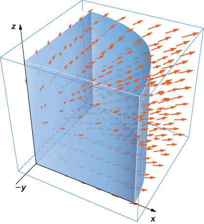
Use the divergence theorem to compute flux integral \({∬}_{S}\text{F}·d\text{S},\) where \(\text{F}(x,y,z)=y\text{j}-z\text{k}\) and S consists of the union of paraboloid \(y={x}^{2}+{z}^{2},0\le y\le 1,\) and disk \({x}^{2}+{z}^{2}\le 1,y=1,\) oriented outward. What is the flux through just the paraboloid?
\({∬}_{D}\text{F}·d\text{S}=\) Net flux \(=0\) ; flux through the paraboloid \(=-\pi\)
Use the divergence theorem to compute flux integral \({∬}_{S}\text{F}·d\text{S},\) where \(\text{F}(x,y,z)=x+y\text{j}+{z}^{4}\text{k}\) and S is a part of cone \(z=\sqrt{{x}^{2}+{y}^{2}}\) beneath top plane \(z=1,\) oriented downward.
Use the divergence theorem to calculate surface integral \({∬}_{S}\text{F}·d\text{S}\) for \(\text{F}(x,y,z)={x}^{4}\text{i}-{x}^{3}{z}^{2}\text{j}+4x{y}^{2}z\text{k},\) where S is the surface inside the cylinder \({x}^{2}+{y}^{2}=1\) between the planes \(z=x+2\,\text{and}\,z=0.\)
\({∬}_{S}\text{F}·d\text{S}=\frac{2\pi }{3}\)
Consider \(\text{F}(x,y,z)={x}^{2}\text{i}+xy\text{j}+(z+1)\text{k}.\) Let E be the solid enclosed by paraboloid \(z=4-{x}^{2}-{y}^{2}\) and plane \(z=0\) with normal vectors pointing outside E. Compute flux F across the boundary of E using the divergence theorem.
For the following exercises, use a CAS along with the divergence theorem to compute the net outward flux for the fields across the given surfaces S.
[T] \(\text{F}=\langle x,-2y,3z\rangle ;\) S is sphere \(\{(x,y,z):{x}^{2}+{y}^{2}+{z}^{2}=6\}.\)
\(16\sqrt{6}\pi\)
[T] \(\text{F}=\langle x,2y,z\rangle ;\) S is the boundary of the tetrahedron in the first octant formed by plane \(x+y+z=1.\)
[T] \(\text{F}=\langle y-2x,{x}^{3}-y,{y}^{2}-z\rangle ;\) S is sphere \(\{(x,y,z):{x}^{2}+{y}^{2}+{z}^{2}=4\}.\)
\(-\frac{128\pi }{3}\)
[T] \(\text{F}=\langle x,y,z\rangle ;\) S is the surface of paraboloid \(z=4-{x}^{2}-{y}^{2},\) for \(z\ge 0,\) plus its base in the xy-plane.
For the following exercises, use a CAS and the divergence theorem to compute the net outward flux for the vector fields across the boundary of the given regions D.
[T] \(\text{F}=\langle z-x,x-y,2y-z\rangle ;\) D is the region between spheres of radius 2 and 4 centered at the origin.
\(-224\pi \approx -703.7168\)
[T] \(\text{F}=\frac{\text{r}}{||\text{r}||}=\frac{\langle x,y,z\rangle }{\sqrt{{x}^{2}+{y}^{2}+{z}^{2}}};\) D is the region between spheres of radius 1 and 2 centered at the origin.
[T] \(\text{F}=\langle {x}^{2},\text{-}{y}^{2},{z}^{2}\rangle ;\) D is the region in the first octant between planes \(z=4-x-y\) and \(z=2-x-y.\)
20
Let \(\text{F}(x,y,z)=2x\text{i}-3xy\text{j}+x{z}^{2}\text{k}.\) Use the divergence theorem to calculate \({∬}_{S}\text{F}·d\text{S},\) where S is the surface of the cube with corners at \((0,0,0),(1,0,0),(0,1,0),\) \((1,1,0),(0,0,1),(1,0,1),(0,1,1),\,\text{and}\,(1,1,1),\) oriented outward.
Use the divergence theorem to find the outward flux of field \(\text{F}(x,y,z)=({x}^{3}-3y)\text{i}+(2yz+1)\text{j}+xyz\text{k}\) through the cube bounded by planes \(x=\pm 1,y=\pm 1,\,\text{and}\,z=\pm 1.\)
\({∬}_{S}\text{F}·d\text{S}=8\)
Let \(\text{F}(x,y,z)=2x\text{i}-3y\text{j}+5z\text{k}\) and let S be hemisphere \(z=\sqrt{9-{x}^{2}-{y}^{2}}\) together with disk \({x}^{2}+{y}^{2}\le 9\) in the xy-plane. Use the divergence theorem to calculate \({∬}_{S} F \cdot dS\) .
Evaluate \({∬}_{S}\text{F}·\text{N}dS,\) where \(\text{F}(x,y,z)={x}^{2}\text{i}+xy\text{j}+{x}^{3}{y}^{3}\text{k}\) and S is the surface consisting of all faces of the tetrahedron bounded by plane \(x+y+z=1\) and the coordinate planes, with outward unit normal vector N.
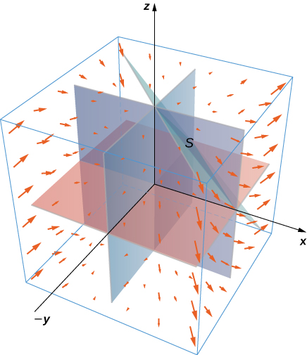
\({∬}_{S}\text{F}·\text{N}dS=\frac{1}{8}\)
Find the net outward flux of field \(\text{F}=\langle bz-cy,cx-az,ay-bx\rangle\) across any smooth closed surface in \({\text{R}}^{3},\) where a, b, and c are constants.
Use the divergence theorem to evaluate \({∬}_{S}\Vert \text{R}\Vert \text{R}·ndS,\) where \(\text{R}(x,y,z)=x\text{i}+y\text{j}+z\text{k}\) and S is sphere \({x}^{2}+{y}^{2}+{z}^{2}={a}^{2},\) with constant \(a>0.\)
\({∬}_{S}\Vert \text{R}\Vert \text{R}·ndS=4\pi {a}^{4}\)
Use the divergence theorem to evaluate \({∬}_{S}\text{F}·d\text{S},\) where \(\text{F}(x,y,z)={y}^{2}z\text{i}+{y}^{3}\text{j}+xz\text{k}\) and S is the boundary of the cube defined by \(-1\le x\le 1,-1\le y\le 1,\,\text{and}\,0\le z\le 2.\)
Let R be the region defined by \({x}^{2}+{y}^{2}+{z}^{2}\le 1.\) Use the divergence theorem to find \({∭}_{R}{z}^{2}dV.\)
\({∭}_{R}{z}^{2}dV=\frac{4\pi }{15}\)
Let E be the solid bounded by the xy-plane and paraboloid \(z=4-{x}^{2}-{y}^{2}\) so that S is the surface of the paraboloid piece together with the disk in the xy-plane that forms its bottom. If \(\text{F}(x,y,z)=(xz\,\text{sin}(yz)+{x}^{3})\text{i}+\text{cos}(yz)\text{j}+(3z{y}^{2}-{e}^{{x}^{2}+{y}^{2}})\text{k},\) find \({∬}_{S}\text{F}·d\text{S}\) using the divergence theorem.
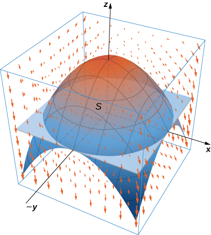
Let E be the solid unit cube with diagonally opposite corners at the origin and (1, 1, 1), and faces parallel to the coordinate planes. Let S be the surface of E, oriented with the outward-pointing normal. Use a CAS to find \({∬}_{S}\text{F}·d\text{S}\) using the divergence theorem if \(\text{F}(x,y,z)=2xy\text{i}+3y{e}^{z}\text{j}+x\,\text{sin}\,z\text{k}.\)
\({∬}_{S}\text{F}·d\text{S}=3e-2+\frac{1}{2}\text{sin}1\approx 6.5759\)
Use the divergence theorem to calculate the flux of \(\text{F}(x,y,z)={x}^{3}\text{i}+{y}^{3}\text{j}+{z}^{3}\text{k}\) through sphere \({x}^{2}+{y}^{2}+{z}^{2}=1.\)
Find \({∬}_{S}\text{F}·d\text{S},\) where \(\text{F}(x,y,z)=x\text{i}+y\text{j}+z\text{k}\) and S is the outwardly oriented surface obtained by removing cube \([1,2]\,\times \,[1,2]\,\times \,[1,2]\) from cube \([0,2]\,\times \,[0,2]\,\times \,[0,2].\)
\({∬}_{S}\text{F}·d\text{S}=21\)
Consider radial vector field \(\text{F}=\frac{\text{r}}{|\text{r}|}=\frac{\langle x,y,z\rangle }{{({x}^{2}+{y}^{2}+{z}^{2})}^{1\text{/}2}}.\) Compute the surface integral, where S is the surface of a sphere of radius a centered at the origin.
Compute the flux of water through parabolic cylinder \(S:y={x}^{2},\) from \(0\le x\le 2,0\le z\le 3,\) if the velocity vector is \(\text{F}(x,y,z)=3{z}^{2}\text{i}+6\text{j}+6xz\text{k}.\)
\({∬}_{S}\text{F}·d\text{S}=72\)
[T] Use a CAS to find the flux of vector field \(\text{F}(x,y,z)=z\text{i}+z\text{j}+\sqrt{{x}^{2}+{y}^{2}}\text{k}\) across the portion of hyperboloid \({x}^{2}+{y}^{2}={z}^{2}+1\) between planes \(z=0\) and \(z=\frac{\sqrt{3}}{3},\) oriented so the unit normal vector points away from the z-axis.
[T] Use a CAS to find the flux of vector field \(\text{F}(x,y,z)=({e}^{y}+x)\text{i}+(3\,\text{cos}(xz)-y)\text{j}+z\text{k}\) through surface S, where S is given by \({z}^{2}=4{x}^{2}+4{y}^{2}\) from \(0\le z\le 4,\) oriented so the unit normal vector points downward.
\({∬}_{S}\text{F}·d\text{S}=-\frac{32\pi }{3}\approx -33.5103\)
[T] Use a CAS to compute \({∬}_{S}\text{F}·d\text{S},\) where \(\text{F}(x,y,z)=x\text{i}+y\text{j}+2z\text{k}\) and S is the boundary of a part of solid sphere \({x}^{2}+{y}^{2}+{z}^{2}\le 2\) with \(0\le z\le 1.\)
Evaluate \({∬}_{S}\text{F}·d\text{S},\) where \(\text{F}(x,y,z)=bx{y}^{2}\text{i}+b{x}^{2}y\text{j}+({x}^{2}+{y}^{2}){z}^{2}\text{k}\) and S is the boundary of the solid cylinder \({x}^{2}+{y}^{2}\le {a}^{2}\) and \(0\le z\le b.\)
\({∬}_{S}\text{F}·d\text{S}=\pi {a}^{4}{b}^{2}\)
[T] Use a CAS to calculate the flux of \(\text{F}(x,y,z)=({x}^{3}+y\,\text{sin}\,z)\text{i}+({y}^{3}+z\,\text{sin}\,x)\text{j}+3z\text{k}\) across surface S, where S is the boundary of the solid bounded by hemispheres \(z=\sqrt{4-{x}^{2}-{y}^{2}}\) and \(z=\sqrt{1-{x}^{2}-{y}^{2}},\) and plane \(z=0.\)
Use the divergence theorem to evaluate \({∬}_{S}\text{F}·d\text{S},\) where \(\text{F}(x,y,z)=xy\text{i}-\frac{1}{2}{y}^{2}\text{j}+z\text{k}\) and S is the surface consisting of three pieces: \(z=4-3{x}^{2}-3{y}^{2},1\le z\le 4\) on the top; \({x}^{2}+{y}^{2}=1,0\le z\le 1\) on the sides; and \(z=0\) on the bottom.
\({∬}_{S}\text{F}·d\text{S}=\frac{5\pi }{2}\)
[T] Use a CAS and the divergence theorem to evaluate \({∬}_{S}\text{F}·d\text{S},\) where \(\text{F}(x,y,z)=(2x+y\,\text{cos}\,z)\text{i}+({x}^{2}-y)\text{j}+{y}^{2}z\text{k}\) and S is sphere \({x}^{2}+{y}^{2}+{z}^{2}=4\) orientated outward.
Use the divergence theorem to evaluate \({∬}_{S}\text{F}·d\text{S},\) where \(\text{F}(x,y,z)=x\text{i}+y\text{j}+z\text{k}\) and S is the boundary of the solid enclosed by paraboloid \(y={x}^{2}+{z}^{2}-2,\) cylinder \({x}^{2}+{z}^{2}=1,\) and plane \(x+y=2,\) and S is oriented outward.
\({∬}_{S}\text{F}·d\text{S}=\frac{21\pi }{2}\)
For the following exercises, Fourier’s law of heat transfer states that the heat flow vector F at a point is proportional to the negative gradient of the temperature; that is, \(\text{F}=\text{-}k∇T,\) which means that heat energy flows hot regions to cold regions. The constant \(k>0\) is called the conductivity, which has metric units of joules per meter per second-kelvin or watts per meter-kelvin. A temperature function for region D is given. Use the divergence theorem to find net outward heat flux \({∬}_{S}\text{F}·\text{N}dS=\text{-}k{∬}_{S}∇T·\text{N}dS\) across the boundary S of D, where \(k=1.\)
\(T(x,y,z)=100+x+2y+z;\) \(D=\{(x,y,z):0\le x\le 1,0\le y\le 1,0\le z\le 1\}\)
\(T(x,y,z)=100+{e}^{\text{-}z};\) \(D=\{(x,y,z):0\le x\le 1,0\le y\le 1,0\le z\le 1\}\)
\({e}^{-1}-1\)
\(T(x,y,z)=100{e}^{\text{-}{x}^{2}-{y}^{2}-{z}^{2}};\) D is the sphere of radius a centered at the origin.
Chapter Review Exercises
True or False? Justify your answer with a proof or a counterexample.
Vector field \(\text{F}(x,y)={x}^{2}y\text{i}+{y}^{2}x\text{j}\) is conservative.
False
For vector field \(\text{F}(x,y)=P(x,y)\text{i}+Q(x,y)\text{j},\) if \({P}_{y}(x,y)={Q}_{x}(x,y)\) in open region \(D,\) then \({∫}_{C}Pdx+Qdy=0.\)
The divergence of a vector field is a vector field.
False
If \(\text{curl}\,\text{F}=0,\) then \(\text{F}\) is a conservative vector field.
Draw the following vector fields.
\(\text{F}(x,y)=\frac{1}{2}\text{i}+2x\text{j}\)
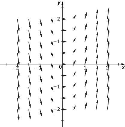
\(\text{F}(x,y)=\frac{<y,3x>}{\sqrt{{x}^{2}+{y}^{2}}}\)
Are the following the vector fields conservative? If so, find the potential function \(f\) such that \(\text{F}=∇f.\)
\(\text{F}(x,y)=y\text{i}+(x-2{e}^{y})\text{j}\)
Conservative, \(f(x,y)=xy-2{e}^{y}\)
\(\text{F}(x,y)=(6xy)\text{i}+(3{x}^{2}-y{e}^{y})\text{j}\)
\(\text{F}(x,y,z)=(2xy+{z}^{2})\text{i}+({x}^{2}+2yz)\text{j}+(2xz+{y}^{2})\text{k}\)
Conservative, \(f(x,y,z)={x}^{2}y+{y}^{2}z+{z}^{2}x\)
\(\text{F}(x,y,z)=({e}^{x}y)\text{i}+({e}^{x}+z)\text{j}+({e}^{x}+{y}^{2})\text{k}\)
Evaluate the following integrals.
\(\underset{C}{∫}{x}^{2}dy+(2x-3xy)dx,\) along \(C:y=\frac{1}{2}x\) from (0, 0) to (4, 2)
\(-\frac{16}{3}\)
\(\underset{C}{∫}ydx+x{y}^{2}dy,\) where \(C:x=\sqrt{t},y=t-1,0\le t\le 1\)
\({∬}_{S}x{y}^{2}dS,\) where S is surface \(z={x}^{2}-y,0\le x\le 1,0\le y\le 4\)
\(\frac{32\sqrt{2}}{9}(3\sqrt{3}-1)\)
Find the divergence and curl for the following vector fields.
\(\text{F}(x,y,z)=3xyz\text{i}+xy{e}^{z}\text{j}-3xy\text{k}\)
\(\text{F}(x,y,z)={e}^{x}\text{i}+{e}^{xy}\text{j}+{e}^{xyz}\text{k}\)
Divergence: \({e}^{x}+x{e}^{xy}+xy{e}^{xyz},\) curl: \(xz{e}^{xyz}\text{i}-yz{e}^{xyz}\text{j}+y{e}^{xy}\text{k}\)
Use Green’s theorem to evaluate the following integrals.
\(\underset{C}{∫}3xydx+2x{y}^{2}dy,\) where C is a square with vertices (0, 0), (0, 2), (2, 2) and (2, 0) oriented counterclockwise.
\({∫}_{C}3ydx+(x+{e}^{y})dy,\) where C is a circle centered at the origin with radius 3
\(-18\pi\)
Use Stokes’ theorem to evaluate \({∬}_{S}\text{curl}\,\text{F}·dS.\)
\(\text{F}(x,y,z)=y\text{i}-x\text{j}+z\text{k},\) where \(S\) is the upper half of the unit sphere
\(\text{F}(x,y,z)=y\text{i}+xyz\text{j}-2zx\text{k},\) where \(S\) is the upward-facing paraboloid \(z={x}^{2}+{y}^{2}\) lying in cylinder \({x}^{2}+{y}^{2}=1\)
\(\text{-}\pi\)
Use the divergence theorem to evaluate \({∬}_{S}\text{F}·dS.\)
\(\text{F}(x,y,z)=({x}^{3}y)\text{i}+(3y-{e}^{x})\text{j}+(z+x)\text{k},\) over cube \(S\) defined by \(-1\le x\le 1,\) \(0\le y\le 2,\) \(0\le z\le 2\)
\(\text{F}(x,y,z)=(2xy)\text{i}+(\text{-}{y}^{2})\text{j}+(2{z}^{3})\text{k},\) where \(S\) is bounded by paraboloid \(z={x}^{2}+{y}^{2}\) and plane \(z=2\)
\(24\pi\)
Find the amount of work performed by a 50-kg woman ascending a helical staircase with radius 2 m and height 100 m. The woman completes five revolutions during the climb. Use 9.8 m/s2 as the acceleration due to gravity.
Find the total mass of a thin wire in the shape of an upper semicircle with radius \(\sqrt{2,}\) and a density function of \(ρ(x,y)=y+{x}^{2}.\)
\(\sqrt{2}(2\sqrt{2}+\pi )=4+\pi \sqrt{2}\)
Find the total mass of a thin sheet in the shape of a hemisphere with radius 2 for \(z\ge 0\) with a density function \(ρ(x,y,z)=x+y+z.\)
Use the divergence theorem to compute the value of the flux integral over the unit sphere with \(\text{F}(x,y,z)=3z\text{i}+2y\text{j}+2x\text{k}.\)
\(8\pi \text{/}3\)
Glossary
- divergence theorem
- a theorem used to transform a difficult flux integral into an easier triple integral and vice versa
- Gauss’ law
- if S is a piecewise, smooth closed surface in a vacuum and Q is the total stationary charge inside of S, then the flux of electrostatic field E across S is \(Q\text{/}{ε}_{0}\)
- inverse-square law
- the electrostatic force at a given point is inversely proportional to the square of the distance from the source of the charge