Section 6.6Surface Integrals
We have seen that a line integral is an integral over a path in a plane or in space. However, if we wish to integrate over a surface (a two-dimensional object) rather than a path (a one-dimensional object) in space, then we need a new kind of integral that can handle integration over objects in higher dimensions. We can extend the concept of a line integral to a surface integral to allow us to perform this integration.
Surface integrals are important for the same reasons that line integrals are important. They have many applications to physics and engineering, and they allow us to develop higher dimensional versions of the Fundamental Theorem of Calculus. In particular, surface integrals allow us to generalize Green’s theorem to higher dimensions, and they appear in some important theorems we discuss in later sections.
Parametric Surfaces
A surface integral is similar to a line integral, except the integration is done over a surface rather than a path. In this sense, surface integrals expand on our study of line integrals. Just as with line integrals, there are two kinds of surface integrals: a surface integral of a scalar-valued function and a surface integral of a vector field.
However, before we can integrate over a surface, we need to consider the surface itself. Recall that to calculate a scalar or vector line integral over curve C, we first need to parameterize C. In a similar way, to calculate a surface integral over surface S, we need to parameterize S. That is, we need a working concept of a parameterized surface (or a parametric surface), in the same way that we already have a concept of a parameterized curve.
A parameterized surface is given by a description of the form
\[\text{r}(u,v)=\langle x(u,v),y(u,v),z(u,v)\rangle .\]
Notice that this parameterization involves two parameters, u and v, because a surface is two-dimensional, and therefore two variables are needed to trace out the surface. The parameters u and v vary over a region called the parameter domain, or parameter space—the set of points in the uv-plane that can be substituted into r. Each choice of u and v in the parameter domain gives a point on the surface, just as each choice of a parameter t gives a point on a parameterized curve. The entire surface is created by making all possible choices of u and v over the parameter domain.
Given a parameterization of surface \(\text{r}(u,v)=\langle x(u,v),y(u,v),z(u,v)\rangle ,\) the parameter domain of the parameterization is the set of points in the uv-plane that can be substituted into r.
Describe surface S parameterized by
\[\text{r}(u,v)=\langle \text{cos}\,u,\text{sin}\,u,v\rangle ,\text{-}\infty <u<\infty ,\text{-}\infty <v<\infty .\]
Hold u constant to see one family of curves, then hold v constant to see the other, and identify the shape each traces.
To get an idea of the shape of the surface, we first plot some points. Since the parameter domain is all of \({ℝ}^{2},\) we can choose any value for u and v and plot the corresponding point. If \(u=v=0,\) then \(\text{r}(0,0)=\langle 1,0,0\rangle ,\) so point (1, 0, 0) is on S. Similarly, points \(\text{r}(\pi ,2)=(-1,0,2)\) and \(\text{r}(\frac{\pi }{2},4)=(0,1,4)\) are on S.
Although plotting points may give us an idea of the shape of the surface, we usually need quite a few points to see the shape. Since it is time-consuming to plot dozens or hundreds of points, we use another strategy. To visualize S, we visualize two families of curves that lie on S. In the first family of curves we hold u constant; in the second family of curves we hold v constant. This allows us to build a “skeleton” of the surface, thereby getting an idea of its shape.
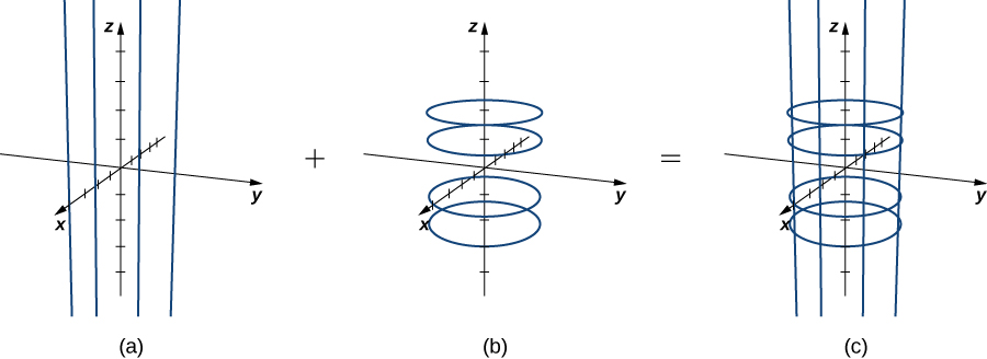
First, suppose that u is a constant K. Then the curve traced out by the parameterization is \(\langle \text{cos}\,K,\text{sin}\,K,v\rangle ,\) which gives a vertical line that goes through point \((\text{cos}\,K,\text{sin}\,K,v)\) in the xy-plane.
Now suppose that v is a constant K. Then the curve traced out by the parameterization is \(\langle \text{cos}\,u,\text{sin}\,u,K\rangle ,\) which gives a circle in plane \(z=K\) with radius 1 and center (0, 0, K).
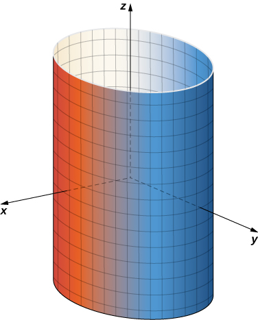
If u is held constant, then we get vertical lines; if v is held constant, then we get circles of radius 1 centered around the vertical line that goes through the origin. Therefore the surface traced out by the parameterization is cylinder \({x}^{2}+{y}^{2}=1\) (Figure 1).
Notice that if \(x=\text{cos}\,u\) and \(y=\text{sin}\,u,\) then \({x}^{2}+{y}^{2}=1,\) so points from S do indeed lie on the cylinder. Conversely, each point on the cylinder is contained in some circle \(\langle \text{cos}\,u,\text{sin}\,u,k\rangle\) for some k, and therefore each point on the cylinder is contained in the parameterized surface (Figure 2).
Notice that if we change the parameter domain, we could get a different surface. For example, if we restricted the domain to \(0\le u\le \pi ,0<v<6,\) then the surface would be a half-cylinder of height 6.
Describe the surface with parameterization \(\text{r}(u,v)=\langle 2\,\text{cos}\,u,2\,\text{sin}\,u,v\rangle ,0\le u<2\pi ,\text{-}\infty <v<\infty .\)
Cylinder \({x}^{2}+{y}^{2}=4\)
It follows from Example 1 that we can parameterize all cylinders of the form \({x}^{2}+{y}^{2}={R}^{2}.\) If S is a cylinder given by equation \({x}^{2}+{y}^{2}={R}^{2},\) then a parameterization of S is
\[\text{r}(u,v)=\langle R\,\text{cos}\,u,R\,\text{sin}\,u,v\rangle ,0\le u<2\pi ,\text{-}\infty <v<\infty .\]
We can also find different types of surfaces given their parameterization, or we can find a parameterization when we are given a surface.
Describe surface S parameterized by
\[\text{r}(u,v)=\langle u\,\text{cos}\,v,u\,\text{sin}\,v,{u}^{2}\rangle ,0\le u<\infty ,0\le v<2\pi .\]
Hold u constant, then v constant, to see the two families of curves, and compute \(x^2+y^2\) in terms of z.
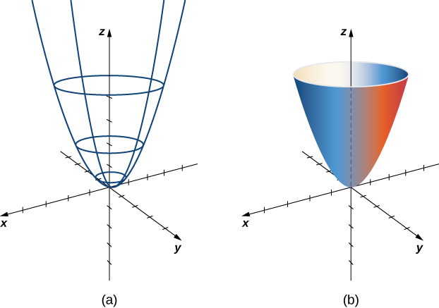
Notice that if u is held constant, then the resulting curve is a circle of radius u in plane \(z={u}^{2}.\) Therefore, as u increases, the radius of the resulting circle increases. If v is held constant, then the resulting curve is a vertical parabola. Therefore, we expect the surface to be an elliptic paraboloid. To confirm this, notice that
\[\begin{array}{ll}{x}^{2}+{y}^{2} & ={(u\,\text{cos}\,v)}^{2}+{(u\,\text{sin}\,v)}^{2} \\ & ={u}^{2}{\text{cos}}^{2}v+{u}^{2}{\text{sin}}^{2}v \\ & ={u}^{2} \\ & =z.\end{array}\]
Therefore, the surface is elliptic paraboloid \({x}^{2}+{y}^{2}=z\) (Figure 3).
Describe the surface parameterized by \(\text{r}(u,v)=\langle u\,\text{cos}\,v,u\,\text{sin}\,v,u\rangle ,\text{-}\infty <u<\infty ,0\le v<2\pi .\)
Cone \({x}^{2}+{y}^{2}={z}^{2}\)
Give a parameterization of the cone \({x}^{2}+{y}^{2}={z}^{2}\) lying on or above the plane \(z=-2.\)
Express the radius of the circular cross-section at height u, then write the point at angle v on that circle.
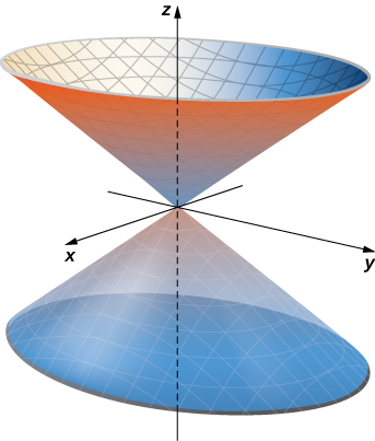
The horizontal cross-section of the cone at height \(z=u\) is circle \({x}^{2}+{y}^{2}={u}^{2}.\) Therefore, a point on the cone at height u has coordinates \((u\,\text{cos}\,v,u\,\text{sin}\,v,u)\) for angle v. Hence, a parameterization of the cone is \(\text{r}(u,v)=\langle u\,\text{cos}\,v,u\,\text{sin}\,v,u\rangle .\) Since we are not interested in the entire cone, only the portion on or above plane \(z=-2,\) the parameter domain is given by \(-2\le u<\infty ,0\le v<2\pi\) (Figure 4).
Give a parameterization for the portion of cone \({x}^{2}+{y}^{2}={z}^{2}\) lying in the first octant.
\(\text{r}(u,v)=\langle u\,\text{cos}\,v,u\,\text{sin}\,v,u\rangle ,\) \(0<u<\infty ,0\le v<\frac{\pi }{2}\)
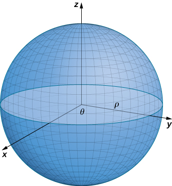
We have discussed parameterizations of various surfaces, but two important types of surfaces need a separate discussion: spheres and graphs of two-variable functions. To parameterize a sphere, it is easiest to use spherical coordinates. The sphere of radius \(ρ\) centered at the origin is given by the parameterization
\[\text{r}(ϕ,θ)=\langle ρ\,\text{cos}\,θ\,\text{sin}\,ϕ,ρ\,\text{sin}\,θ\,\text{sin}\,ϕ,ρ\,\text{cos}\,ϕ\rangle ,0\le θ\le 2\pi ,0\le ϕ\le \pi .\]
The idea of this parameterization is that as \(ϕ\) sweeps downward from the positive z-axis, a circle of radius \(ρ\,\text{sin}\,ϕ\) is traced out by letting \(θ\) run from 0 to \(2\pi .\) To see this, let \(ϕ\) be fixed. Then
\[\begin{array}{ll}{x}^{2}+{y}^{2} & ={(ρ\,\text{cos}\,θ\,\text{sin}\,ϕ)}^{2}+{(ρ\,\text{sin}\,θ\,\text{sin}\,ϕ)}^{2} \\ & ={ρ}^{2}{\text{sin}}^{2}ϕ({\text{cos}}^{2}θ+{\text{sin}}^{2}θ) \\ & ={ρ}^{2}{\text{sin}}^{2}ϕ \\ & ={(ρ\,\text{sin}\,ϕ)}^{2}.\end{array}\]
This results in the desired circle (Figure 5).
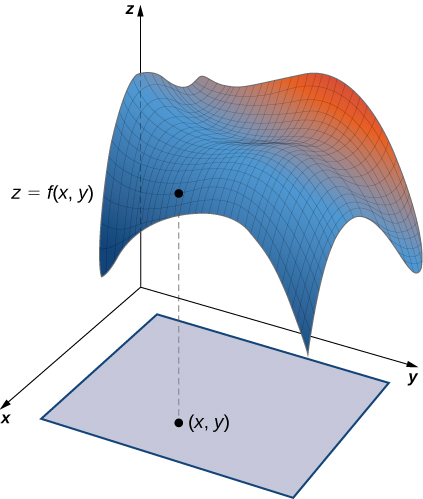
Finally, to parameterize the graph of a two-variable function, we first let \(z=f(x,y)\) be a function of two variables. The simplest parameterization of the graph of \(f\) is \(\text{r}(x,y)=\langle x,y,f(x,y)\rangle ,\) where x and y vary over the domain of \(f\) (Figure 6). For example, the graph of \(f(x,y)={x}^{2}y\) can be parameterized by \(\text{r}(x,y)=\langle x,y,{x}^{2}y\rangle ,\) where the parameters x and y vary over the domain of \(f.\) If we only care about a piece of the graph of \(f\) —say, the piece of the graph over rectangle \([1,3]\,\times \,[2,5]\) —then we can restrict the parameter domain to give this piece of the surface:
\[\text{r}(x,y)=\langle x,y,{x}^{2}y\rangle ,1\le x\le 3,2\le y\le 5.\]
Similarly, if S is a surface given by equation \(x=g(y,z)\) or equation \(y=h(x,z),\) then a parameterization of S is
\(\text{r}(y,z)=\langle g(y,z),y,z\rangle\) or \(\text{r}(x,z)=\langle x,h(x,z),z\rangle ,\) respectively. For example, the graph of paraboloid \(2y={x}^{2}+{z}^{2}\) can be parameterized by \(\text{r}(x,z)=\langle x,\frac{{x}^{2}+{z}^{2}}{2},z\rangle ,0\le x<\infty ,0\le z<\infty .\) Notice that we do not need to vary over the entire domain of y because x and z are squared.
Let’s now generalize the notions of smoothness and regularity to a parametric surface. Recall that curve parameterization \(\text{r}(t),a\le t\le b\) is regular if \(\text{r}\prime (t)\ne 0\) for all t in \([a,b].\) For a curve, this condition ensures that the image of r really is a curve, and not just a point. For example, consider curve parameterization \(\text{r}(t)=\langle 1,2\rangle ,0\le t\le 5.\) The image of this parameterization is simply point \((1,2),\) which is not a curve. Notice also that \(\text{r}\prime (t)=0.\) The fact that the derivative is the zero vector indicates we are not actually looking at a curve.
Analogously, we would like a notion of regularity for surfaces so that a surface parameterization really does trace out a surface. To motivate the definition of regularity of a surface parameterization, consider parameterization
\[\text{r}(u,v)=\langle 0,\text{cos}\,v,1\rangle ,0\le u\le 1,0\le v\le \pi .\]
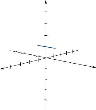
Although this parameterization appears to be the parameterization of a surface, notice that the image is actually a line (Figure 7). How could we avoid parameterizations such as this? Parameterizations that do not give an actual surface? Notice that \({\text{r}}_{u}=\langle 0,0,0\rangle\) and \({\text{r}}_{v}=\langle 0,\text{-}\text{sin}\,v,0\rangle ,\) and the corresponding cross product is zero. The analog of the condition \(\text{r}\prime (t)=0\) is that \({\text{r}}_{u}\,\times \,{\text{r}}_{v}\) is not zero for any point \((u,v)\) in the parameter domain, which is a regular parameterization.
Parameterization \(\text{r}(u,v)=\langle x(u,v),y(u,v),z(u,v)\rangle\) is a regular parameterization if \({\text{r}}_{u}\,\times \,{\text{r}}_{v}\) is not zero for any point \((u,v)\) in the parameter domain.
If parameterization r is regular, then the image of r is a two-dimensional object, as a surface should be. Throughout this chapter, parameterizations \(\text{r}(u,v)=\langle x(u,v),y(u,v),z(u,v)\rangle\) are assumed to be regular.
Recall that curve parameterization \(\text{r}(t),a\le t\le b\) is smooth if \(\text{r}\prime (t)\) is continuous and \(\text{r}\prime (t)\ne 0\) for all t in \([a,b].\) Informally, a curve parameterization is smooth if the resulting curve has no sharp corners. The definition of a smooth surface parameterization is similar. Informally, a surface parameterization is smooth if the resulting surface has no sharp corners.
A surface parameterization \(\text{r}(u,v)=\langle x(u,v),y(u,v),z(u,v)\rangle\) is smooth if vector \({\text{r}}_{u}\,\times \,{\text{r}}_{v}\) is not zero for any choice of u and v in the parameter domain.
A surface may also be piecewise smooth if it has smooth faces but also has locations where the directional derivatives do not exist.
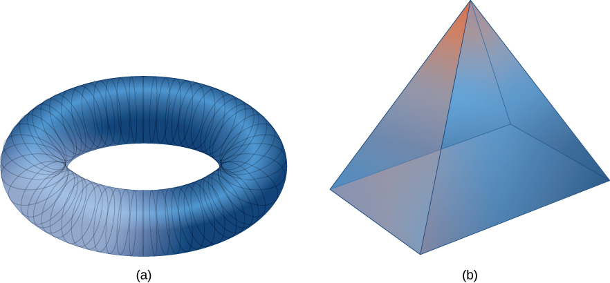
Which of the figures in Figure 8 is smooth?
Find a parameterization for the torus, compute \({\text{r}}_{u}\times{\text{r}}_{v}\), and check whether it is ever the zero vector.
The surface in Figure 8(a) can be parameterized by
\[\text{r}(u,v)=\langle (2+\text{cos}\,v)\text{cos}\,u,(2+\text{cos}\,v)\text{sin}\,u,\text{sin}\,v\rangle ,0\le u<2\pi ,0\le v<2\pi \]
(we can use technology to verify). Notice that vectors
\[{\text{r}}_{u}=\langle \text{-}(2+\text{cos}\,v)\text{sin}\,u,(2+\text{cos}\,v)\text{cos}\,u,0\rangle \,\text{and}\,{\text{r}}_{v}=\langle \text{-}\text{sin}\,v\,\text{cos}\,u,\text{-}\text{sin}\,v\,\text{sin}\,u,\text{cos}\,v\rangle \]
exist for any choice of u and v in the parameter domain, and
\[\begin{array}{ll}{\text{r}}_{u}\,\times \,{\text{r}}_{v} & =|\begin{array}{lll}\text{i} & \text{j} & \text{k} \\ \text{-}(2+\text{cos}\,v)\text{sin}\,u & (2+\text{cos}\,v)\text{cos}\,u & 0 \\ \text{-}\text{sin}\,v\,\text{cos}\,u & \text{-}\text{sin}\,v\,\text{sin}\,u & \text{cos}\,v\end{array}| \\ & =[(2+\text{cos}\,v)\text{cos}\,u\,\text{cos}\,v]\text{i}+[(2+\text{cos}\,v)\text{sin}\,u\,\text{cos}\,v]\text{j} \\ & \,+[(2+\text{cos}\,v)\text{sin}\,v\,{\text{sin}}^{2}u+(2+\text{cos}\,v)\text{sin}\,v\,{\text{cos}}^{2}u]\text{k} \\ & =[(2+\text{cos}\,v)\text{cos}\,u\,\text{cos}\,v]\text{i}+[(2+\text{cos}\,v)\text{sin}\,u\,\text{cos}\,v]\text{j}+[(2+\text{cos}\,v)\text{sin}\,v]\text{k}.\end{array}\]
The k component of this vector is zero only if \(v=0\) or \(v=\pi .\) If \(v=0\) or \(v=\pi ,\) then the only choices for u that make the j component zero are \(u=0\) or \(u=\pi .\) But, these choices of u do not make the i component zero. Therefore, \({\text{r}}_{u}\,\times \,{\text{r}}_{v}\) is not zero for any choice of u and v in the parameter domain, and the parameterization is smooth. Notice that the corresponding surface has no sharp corners.
In the pyramid in Figure 8(b), the sharpness of the corners ensures that directional derivatives do not exist at those locations. Therefore, the pyramid has no smooth parameterization. However, the pyramid consists of five smooth faces, and thus this surface is piecewise smooth.
Is the surface parameterization \(\text{r}(u,v)=\langle {u}^{2v},v+1,\text{sin}\,u\rangle ,0\le u\le 2,0\le v\le 3\) smooth?
Yes
Surface Area of a Parametric Surface
Our goal is to define a surface integral, and as a first step we have examined how to parameterize a surface. The second step is to define the surface area of a parametric surface. The notation needed to develop this definition is used throughout the rest of this chapter.
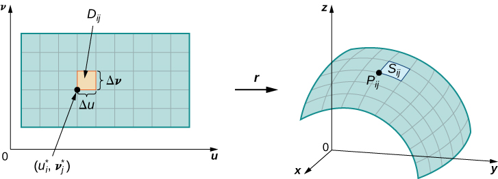
Let S be a surface with parameterization \(\text{r}(u,v)=\langle x(u,v),y(u,v),z(u,v)\rangle\) over some parameter domain D. We assume here and throughout that the surface parameterization \(\text{r}(u,v)=\langle x(u,v),y(u,v),z(u,v)\rangle\) is continuously differentiable—meaning, each component function has continuous partial derivatives. Assume for the sake of simplicity that D is a rectangle (although the following material can be extended to handle nonrectangular parameter domains). Divide rectangle D into subrectangles \({D}_{ij}\) with horizontal width \(\Delta u\) and vertical length \(\Delta v.\) Suppose that i ranges from 1 to m and j ranges from 1 to n so that D is subdivided into mn rectangles. This division of D into subrectangles gives a corresponding division of surface S into pieces \({S}_{ij}.\) Choose point \({P}_{ij}\) in each piece \({S}_{ij}.\) Point \({P}_{ij}\) corresponds to point \(({u}_{i},{v}_{j})\) in the parameter domain.
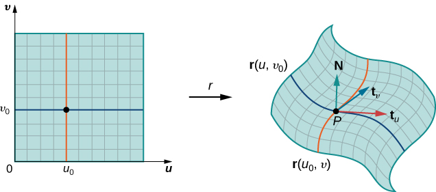
Note that we can form a grid with lines that are parallel to the u-axis and the v-axis in the uv-plane. These grid lines correspond to a set of grid curves on surface S that is parameterized by \(\text{r}(u,v).\) Without loss of generality, we assume that \({P}_{ij}\) is located at the corner of two grid curves, as in Figure 9. If we think of r as a mapping from the uv-plane to \({ℝ}^{3},\) the grid curves are the image of the grid lines under r. To be precise, consider the grid lines that go through point \(({u}_{i},{v}_{j}).\) One line is given by \(x={u}_{i},y=v;\) the other is given by \(x=u,y={v}_{j}.\) In the first grid line, the horizontal component is held constant, yielding a vertical line through \(({u}_{i},{v}_{j}).\) In the second grid line, the vertical component is held constant, yielding a horizontal line through \(({u}_{i},{v}_{j}).\) The corresponding grid curves are \(\text{r}({u}_{i},v)\) and \(\text{r}(u,{v}_{j}),\) and these curves intersect at point \({P}_{ij}.\)
Now consider the vectors that are tangent to these grid curves. For grid curve \(\text{r}({u}_{i},v),\) the tangent vector at \({P}_{ij}\) is
\[{\text{t}}_{v}({P}_{ij})={\text{r}}_{v}({u}_{i},{v}_{j})=\langle {x}_{v}({u}_{i},{v}_{j}),{y}_{v}({u}_{i},{v}_{j}),{z}_{v}({u}_{i},{v}_{j})\rangle .\]
For grid curve \(\text{r}(u,{v}_{j}),\) the tangent vector at \({P}_{ij}\) is
\[{\text{t}}_{u}({P}_{ij})={\text{r}}_{u}({u}_{i},{v}_{j})=\langle {x}_{u}({u}_{i},{v}_{j}),{y}_{u}({u}_{i},{v}_{j}),{z}_{u}({u}_{i},{v}_{j})\rangle .\]
If vector \(\text{N}={\text{t}}_{u}({P}_{ij})\,\times \,{\text{t}}_{v}({P}_{ij})\) exists and is not zero, then the tangent plane at \({P}_{ij}\) exists (Figure 10). If piece \({S}_{ij}\) is small enough, then the tangent plane at point \({P}_{ij}\) is a good approximation of piece \({S}_{ij}.\)
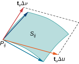
The tangent plane at \({P}_{ij}\) contains vectors \({\text{t}}_{u}({P}_{ij})\) and \({\text{t}}_{v}({P}_{ij}),\) and therefore the parallelogram spanned by \({\text{t}}_{u}({P}_{ij})\) and \({\text{t}}_{v}({P}_{ij})\) is in the tangent plane. Since the original rectangle in the uv-plane corresponding to \({S}_{ij}\) has width \(\Delta u\) and length \(\Delta v,\) the parallelogram that we use to approximate \({S}_{ij}\) is the parallelogram spanned by \(\Delta u{\text{t}}_{u}({P}_{ij})\) and \(\Delta v{\text{t}}_{v}({P}_{ij}).\) In other words, we scale the tangent vectors by the constants \(\Delta u\) and \(\Delta v\) to match the scale of the original division of rectangles in the parameter domain. Therefore, the area of the parallelogram used to approximate the area of \({S}_{ij}\) is
\[\Delta {S}_{ij}\approx \Vert (\Delta u{\text{t}}_{u}({P}_{ij}))\,\times \,(\Delta v{\text{t}}_{v}({P}_{ij}))\Vert =\Vert {\text{t}}_{u}({P}_{ij})\,\times \,{\text{t}}_{v}({P}_{ij})\Vert \Delta u\Delta v.\]
Varying point \({P}_{ij}\) over all pieces \({S}_{ij}\) and the previous approximation leads to the following definition of surface area of a parametric surface (Figure 11).
Let \(\text{r}(u,v)=\langle x(u,v),y(u,v),z(u,v)\rangle\) with parameter domain D be a smooth parameterization of surface S. Furthermore, assume that S is traced out only once as \((u,v)\) varies over D. The surface area of S is
\[{∬}_{D}\Vert {\text{t}}_{u}\,\times \,{\text{t}}_{v}\Vert dA,\]
where \({\text{t}}_{u}=\langle \frac{∂x}{∂u},\frac{∂y}{∂u},\frac{∂z}{∂u}\rangle\) and \({\text{t}}_{v}=\langle \frac{∂x}{∂v},\frac{∂y}{∂v},\frac{∂z}{∂v}\rangle\) and all partial derivatives are continuous.
Calculate the lateral surface area (the area of the “side,” not including the base) of the right circular cone with height h and radius r.
Set up a parameterization \(\text{s}(u,v)\) for the cone using slope \(k=\tan\alpha\), then compute \({\text{t}}_u\times{\text{t}}_v\) and its magnitude.
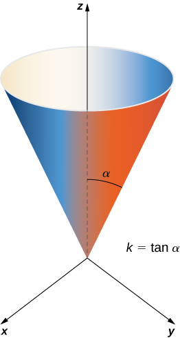
Before calculating the surface area of this cone using Equation 16, we need a parameterization. We assume this cone is in \({ℝ}^{3}\) with its vertex at the origin (Figure 12). To obtain a parameterization, let \(α\) be the angle that is swept out by starting at the positive z-axis and ending at the cone, and let \(k=\text{tan}\,α.\) For a height value v with \(0\le v\le h,\) the radius of the circle formed by intersecting the cone with plane \(z=v\) is \(kv.\) Therefore, a parameterization of this cone is
\[\text{s}(u,v)=\langle kv\,\text{cos}\,u,kv\,\text{sin}\,u,v\rangle ,0\le u<2\pi ,0\le v\le h.\]
The idea behind this parameterization is that for a fixed v value, the circle swept out by letting u vary is the circle at height v and radius kv. As v increases, the parameterization sweeps out a “stack” of circles, resulting in the desired cone.
With a parameterization in hand, we can calculate the surface area of the cone using Equation 16. The tangent vectors are \({\text{t}}_{u}=\langle \text{-}kv\,\text{sin}\,u,kv\,\text{cos}\,u,0\rangle\) and \({\text{t}}_{v}=\langle k\,\text{cos}\,u,k\,\text{sin}\,u,1\rangle .\) Therefore,
\[\begin{array}{ll}{\text{t}}_{u}\,\times \,{\text{t}}_{v} & =|\begin{array}{lll}\text{i} & \text{j} & \text{k} \\ \text{-}kv\,\text{sin}\,u & kv\,\text{cos}\,u & 0 \\ k\,\text{cos}\,u & k\,\text{sin}\,u & 1\end{array}| \\ & =\langle kv\,\text{cos}\,u,kv\,\text{sin}\,u,\text{-}{k}^{2}v\,{\text{sin}}^{2}u-{k}^{2}v\,{\text{cos}}^{2}u\rangle \\ & =\langle kv\,\text{cos}\,u,kv\,\text{sin}\,u,\text{-}{k}^{2}v\rangle .\end{array}\]
The magnitude of this vector is
\[\begin{array}{ll}\Vert \langle kv\,\text{cos}\,u,kv\,\text{sin}\,u,\text{-}{k}^{2}v\rangle \Vert & =\sqrt{{k}^{2}{v}^{2}{\text{cos}}^{2}u+{k}^{2}{v}^{2}{\text{sin}}^{2}u+{k}^{4}{v}^{2}} \\ & =\sqrt{{k}^{2}{v}^{2}+{k}^{4}{v}^{2}} \\ & =kv\sqrt{1+{k}^{2}}.\end{array}\]
By Equation 16, the surface area of the cone is
\[\begin{array}{ll}{∬}_{D}\Vert {\text{t}}_{u}\,\times \,{\text{t}}_{v}\Vert dA & ={∫}_{0}^{h}{∫}_{0}^{2\pi }kv\sqrt{1+{k}^{2}}dudv \\ & =2\pi k\sqrt{1+{k}^{2}}{∫}_{0}^{h}vdv \\ & =2\pi k\sqrt{1+{k}^{2}}{[\frac{{v}^{2}}{2}]}_{0}^{h} \\ & =\pi k{h}^{2}\sqrt{1+{k}^{2}}.\end{array}\]
Since \(k=\text{tan}\,α=r\text{/}h,\)
\[\begin{array}{ll}\pi k{h}^{2}\sqrt{1+{k}^{2}} & =\pi \frac{r}{h}{h}^{2}\sqrt{1+\frac{{r}^{2}}{{h}^{2}}} \\ & =\pi rh\sqrt{1+\frac{{r}^{2}}{{h}^{2}}} \\ & =\pi r\sqrt{{h}^{2}+{h}^{2}(\frac{{r}^{2}}{{h}^{2}})} \\ & =\pi r\sqrt{{h}^{2}+{r}^{2}}.\end{array}\]
Therefore, the lateral surface area of the cone is \(\pi r\sqrt{{h}^{2}+{r}^{2}}.\)
The surface area of a right circular cone with radius r and height h is usually given as \(\pi {r}^{2}+\pi r\sqrt{{h}^{2}+{r}^{2}}.\) The reason for this is that the circular base is included as part of the cone, and therefore the area of the base \(\pi {r}^{2}\) is added to the lateral surface area \(\pi r\sqrt{{h}^{2}+{r}^{2}}\) that we found.
Find the surface area of the surface with parameterization \(\text{r}(u,v)=\langle u+v,{u}^{2},2v\rangle ,0\le u\le 3,0\le v\le 2.\)
\(\approx 43.02\)
Show that the surface area of the sphere \({x}^{2}+{y}^{2}+{z}^{2}={r}^{2}\) is \(4\pi {r}^{2}.\)
Use the standard spherical parameterization, compute \({\text{t}}_{\phi}\times{\text{t}}_{\theta}\) and its magnitude, then integrate over the parameter domain.
The sphere has parameterization
\[\langle r\,\text{cos}\,θ\,\text{sin}\,ϕ,r\,\text{sin}\,θ\,\text{sin}\,ϕ,r\,\text{cos}\,ϕ\rangle ,0\le θ<2\pi ,0\le ϕ\le \pi .\]
The tangent vectors are
\[{\text{t}}_{θ}=\langle \text{-}r\,\text{sin}\,θ\,\text{sin}\,ϕ,r\,\text{cos}\,θ\,\text{sin}\,ϕ,0\rangle \,\text{and}\,{\text{t}}_{ϕ}=\langle r\,\text{cos}\,θ\,\text{cos}\,ϕ,r\,\text{sin}\,θ\,\text{cos}\,ϕ,\text{-}r\,\text{sin}\,ϕ\rangle .\]
Therefore,
\[\begin{array}{ll}{\text{t}}_{ϕ}\,\times \,{\text{t}}_{θ} & =\langle {r}^{2}\text{cos}\,θ\,{\text{sin}}^{2}ϕ,{r}^{2}\text{sin}\,θ\,{\text{sin}}^{2}ϕ,{r}^{2}{\text{sin}}^{2}θ\,\text{sin}\,ϕ\,\text{cos}\,ϕ+{r}^{2}{\text{cos}}^{2}θ\,\text{sin}\,ϕ\,\text{cos}\,ϕ\rangle \\ & =\langle {r}^{2}\text{cos}\,θ\,{\text{sin}}^{2}ϕ,{r}^{2}\text{sin}\,θ\,{\text{sin}}^{2}ϕ,{r}^{2}\text{sin}\,ϕ\,\text{cos}\,ϕ\rangle .\end{array}\]
Now,
\[\begin{array}{ll}\Vert {\text{t}}_{ϕ}\,\times \,{\text{t}}_{θ}\Vert & =\sqrt{{r}^{4}{\text{sin}}^{4}ϕ\,{\text{cos}}^{2}θ+{r}^{4}{\text{sin}}^{4}ϕ\,{\text{sin}}^{2}θ+{r}^{4}{\text{sin}}^{2}ϕ\,{\text{cos}}^{2}ϕ} \\ & =\sqrt{{r}^{4}{\text{sin}}^{4}ϕ+{r}^{4}{\text{sin}}^{2}ϕ\,{\text{cos}}^{2}ϕ} \\ & ={r}^{2}\sqrt{{\text{sin}}^{2}ϕ} \\ & ={r}^{2}\,\text{sin}\,ϕ.\end{array}\]
Notice that \(\text{sin}\,ϕ\ge 0\) on the parameter domain because \(0\le ϕ<\pi ,\) and this justifies equation \(\sqrt{{\text{sin}}^{2}ϕ}=\text{sin}\,ϕ.\) The surface area of the sphere is
\[{∫}_{0}^{2\pi }{∫}_{0}^{\pi }{r}^{2}\text{sin}\,ϕdϕdθ={r}^{2}{∫}_{0}^{2\pi }2dθ=4\pi {r}^{2}.\]
We have derived the familiar formula for the surface area of a sphere using surface integrals.
Show that the surface area of cylinder \({x}^{2}+{y}^{2}={r}^{2},0\le z\le h\) is \(2\pi rh.\) Notice that this cylinder does not include the top and bottom circles.
With the standard parameterization of a cylinder, Equation 16 shows that the surface area is \(2\pi rh.\)
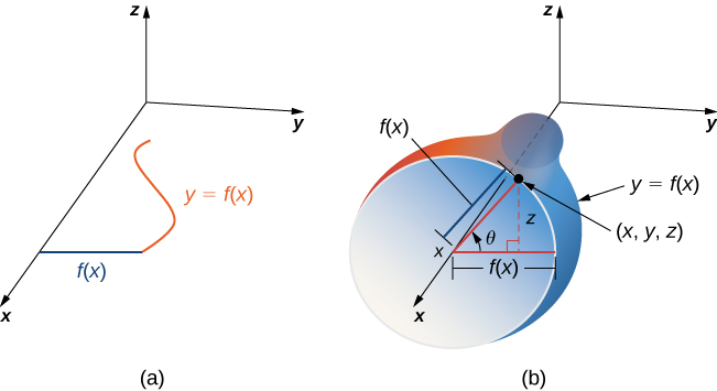
In addition to parameterizing surfaces given by equations or standard geometric shapes such as cones and spheres, we can also parameterize surfaces of revolution. Therefore, we can calculate the surface area of a surface of revolution by using the same techniques. Let \(y=f(x)\ge 0\) be a positive single-variable function on the domain \(a\le x\le b\) and let S be the surface obtained by rotating \(f\) about the x-axis (Figure 13). Let \(θ\) be the angle of rotation. Then, S can be parameterized with parameters x and \(θ\) by
\[\text{r}(x,θ)=\langle x,f(x)\text{cos}\,θ,f(x)\text{sin}\,θ\rangle ,a\le x\le b,0\le θ<2\pi .\]
Find the area of the surface of revolution obtained by rotating \(y={x}^{2},0\le x\le b\) about the x-axis (Figure 14).
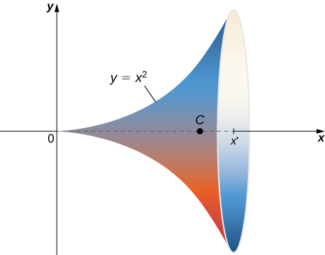
Use the surface-of-revolution parameterization \(\text{r}(x,\theta)\), compute \({\text{t}}_x\times{\text{t}}_\theta\) and its magnitude, then integrate.
This surface has parameterization
\[\text{r}(x,θ)=\langle x,{x}^{2}\text{cos}\,θ,{x}^{2}\text{sin}\,θ\rangle ,0\le x\le b,0\le θ<2\pi .\]
The tangent vectors are \({\text{t}}_{x}=\langle 1,2x\,\text{cos}\,θ,2x\,\text{sin}\,θ\rangle \,\text{and}\,{\text{t}}_{θ}=\langle 0,\text{-}{x}^{2}\text{sin}\,θ,{x}^{2}\text{cos}\,θ\rangle .\) Therefore,
\[\begin{array}{ll}{\text{t}}_{x}\,\times \,{\text{t}}_{θ} & =\langle 2{x}^{3}{\text{cos}}^{2}θ+2{x}^{3}{\text{sin}}^{2}θ,\text{-}{x}^{2}\text{cos}\,θ,\text{-}{x}^{2}\text{sin}\,θ\rangle \\ & =\langle 2{x}^{3},\text{-}{x}^{2}\text{cos}\,θ,\text{-}{x}^{2}\text{sin}\,θ\rangle \end{array}\]
and
\[\begin{array}{ll}||{\text{t}}_{x}\,\times \,{\text{t}}_{θ}|| & =\sqrt{4{x}^{6}+{x}^{4}{\text{cos}}^{2}θ+{x}^{4}{\text{sin}}^{2}θ} \\ & =\sqrt{4{x}^{6}+{x}^{4}} \\ & ={x}^{2}\sqrt{4{x}^{2}+1}.\end{array}\]
The area of the surface of revolution is
\[\begin{array}{ll}{∫}_{0}^{b}{∫}_{0}^{\pi }{x}^{2}\sqrt{4{x}^{2}+1}dθdx & =2\pi {∫}_{0}^{b}{x}^{2}\sqrt{4{x}^{2}+1}dx \\ & =2\pi {[\frac{1}{64}(2\sqrt{4{x}^{2}+1}(8{x}^{3}+x){-\text{sinh}}^{-1}(2x))]}_{0}^{b} \\ & =2\pi [\frac{1}{64}(2\sqrt{4{b}^{2}+1}(8{b}^{3}+b){-\text{sinh}}^{-1}(2b))].\end{array}\]
Use Equation 16 to find the area of the surface of revolution obtained by rotating curve \(y=\text{sin}\,x,0\le x\le \pi\) about the x-axis.
\(2\pi (\sqrt{2}+{\text{sinh}}^{-1}(1))\)
Surface Integral of a Scalar-Valued Function
Now that we can parameterize surfaces and we can calculate their surface areas, we are able to define surface integrals. First, let’s look at the surface integral of a scalar-valued function. Informally, the surface integral of a scalar-valued function is an analog of a scalar line integral in one higher dimension. The domain of integration of a scalar line integral is a parameterized curve (a one-dimensional object); the domain of integration of a scalar surface integral is a parameterized surface (a two-dimensional object). Therefore, the definition of a surface integral follows the definition of a line integral quite closely. For scalar line integrals, we chopped the domain curve into tiny pieces, chose a point in each piece, computed the function at that point, and took a limit of the corresponding Riemann sum. For scalar surface integrals, we chop the domain region (no longer a curve) into tiny pieces and proceed in the same fashion.
Let S be a piecewise smooth surface with parameterization \(\text{r}(u,v)=\langle x(u,v),y(u,v),z(u,v)\rangle\) with parameter domain D and let \(f(x,y,z)\) be a function with a domain that contains S. For now, assume the parameter domain D is a rectangle, but we can extend the basic logic of how we proceed to any parameter domain (the choice of a rectangle is simply to make the notation more manageable). Divide rectangle D into subrectangles \({D}_{ij}\) with horizontal width \(\Delta u\) and vertical length \(\Delta v.\) Suppose that i ranges from 1 to m and j ranges from 1 to n so that D is subdivided into mn rectangles. This division of D into subrectangles gives a corresponding division of S into pieces \({S}_{ij}.\) Choose point \({P}_{ij}\) in each piece \({S}_{ij},\) evaluate \({P}_{ij}\) at \(f\) , and multiply by area \(\Delta {S}_{ij}\) to form the Riemann sum
\[\sum_{i=1}^{m}\sum_{j=1}^{n}f({P}_{ij})\Delta {S}_{ij}.\]
To define a surface integral of a scalar-valued function, we let the areas of the pieces of S shrink to zero by taking a limit.
The surface integral of a scalar-valued function of \(f\) over a piecewise smooth surface S is
\[\underset{S}{∬}f(x,y,z)dS=\underset{m,n\to \infty }{\text{lim}}\sum_{i=1}^{m}\sum_{j=1}^{n}f({P}_{ij})\Delta {S}_{ij}.\]
Again, notice the similarities between this definition and the definition of a scalar line integral. In the definition of a line integral we chop a curve into pieces, evaluate a function at a point in each piece, and let the length of the pieces shrink to zero by taking the limit of the corresponding Riemann sum. In the definition of a surface integral, we chop a surface into pieces, evaluate a function at a point in each piece, and let the area of the pieces shrink to zero by taking the limit of the corresponding Riemann sum. Thus, a surface integral is similar to a line integral but in one higher dimension.
The definition of a scalar line integral can be extended to parameter domains that are not rectangles by using the same logic used earlier. The basic idea is to chop the parameter domain into small pieces, choose a sample point in each piece, and so on. The exact shape of each piece in the sample domain becomes irrelevant as the areas of the pieces shrink to zero.
Scalar surface integrals are difficult to compute from the definition, just as scalar line integrals are. To develop a method that makes surface integrals easier to compute, we approximate surface areas \(\Delta {S}_{ij}\) with small pieces of a tangent plane, just as we did in the previous subsection. Recall the definition of vectors \({\text{t}}_{u}\) and \({\text{t}}_{v}\text{:}\)
\[{\text{t}}_{u}=\langle \frac{∂x}{∂u},\frac{∂y}{∂u},\frac{∂z}{∂u}\rangle \,\text{and}\,{\text{t}}_{v}=\langle \frac{∂x}{∂v},\frac{∂y}{∂v},\frac{∂z}{∂v}\rangle .\]
From the material we have already studied, we know that
\[\Delta {S}_{ij}\approx \Vert {\text{t}}_{u}({P}_{ij})\,\times \,{\text{t}}_{v}({P}_{ij})\Vert \Delta u\Delta v.\]
Therefore,
\[{∬}_{S}f(x,y,z)dS\approx \underset{m,n\to \infty }{\text{lim}}\sum_{i=1}^{m}\sum_{j=1}^{n}f({P}_{ij})\Vert {\text{t}}_{u}({P}_{ij})\,\times \,{\text{t}}_{v}({P}_{ij})\Vert \Delta u\Delta v.\]
This approximation becomes arbitrarily close to \(\underset{m,n\to \infty }{\text{lim}}\sum_{i=1}^{m}\sum_{j=1}^{n}f({P}_{ij})\Delta {S}_{ij}\) as we increase the number of pieces \({S}_{ij}\) by letting m and n go to infinity. Therefore, we have the following equation to calculate scalar surface integrals:
\[{∬}_{S}f(x,y,z)dS=\underset{D}{∬}f(\text{r}(u,v))\Vert {\text{t}}_{u}\,\times \,{\text{t}}_{v}\Vert dA.\]
Equation 37 allows us to calculate a surface integral by transforming it into a double integral. This equation for surface integrals is analogous to (see original) for line integrals:
\[{∫}_{C}f(x,y,z)ds={∫}_{a}^{b}f(\text{r}(t))\Vert {r}^{\prime }(t)\Vert dt.\]
In this case, vector \({\text{t}}_{u}\,\times \,{\text{t}}_{v}\) is perpendicular to the surface, whereas vector \({r}^{\prime }(t)\) is tangent to the curve.
Calculate surface integral \({∬}_{S}5dS,\) where \(S\) is the surface with parameterization \(\text{r}(u,v)=\langle u,{u}^{2},v\rangle\) for \(0\le u\le 2\) and \(0\le v\le u.\)
Compute \({\text{t}}_u\times{\text{t}}_v\) and its magnitude, then set up the double integral over the triangular parameter domain.
Notice that this parameter domain D is a triangle, and therefore the parameter domain is not rectangular. This is not an issue though, because Equation 37 does not place any restrictions on the shape of the parameter domain.
To use Equation 37 to calculate the surface integral, we first find vector \({\text{t}}_{u}\) and \({\text{t}}_{v}.\) Note that \({\text{t}}_{u}=\langle 1,2u,0\rangle\) and \({\text{t}}_{v}=\langle 0,0,1\rangle .\) Therefore,
\[{\text{t}}_{u}\,\times \,{\text{t}}_{v}=|\begin{array}{lll}\text{i} & \text{j} & \text{k} \\ 1 & 2u & 0 \\ 0 & 0 & 1\end{array}|=\langle 2u,-1,0\rangle \]
and
\[\Vert {\text{t}}_{u}\,\times \,{\text{t}}_{v}\Vert =\sqrt{1+4{u}^{2}}.\]
By Equation 37,
\[\begin{array}{ll}{∬}_{S}5dS & =5{∬}_{D}\sqrt{1+4{u}^{2}}dA \\ & =5{∫}_{0}^{2}{∫}_{0}^{u}\sqrt{1+4{u}^{2}}dvdu=5{∫}_{0}^{2}u\sqrt{1+4{u}^{2}}du \\ & =5{[\frac{{(1+4{u}^{2})}^{3\text{/}2}}{3}]}_{0}^{2}=\frac{5({17}^{3\text{/}2}-1)}{12}\approx 28.79.\end{array}\]
Calculate surface integral \({∬}_{S}(x+{y}^{2})dS,\) where S is cylinder \({x}^{2}+{y}^{2}=4,0\le z\le 3\) (Figure 15).
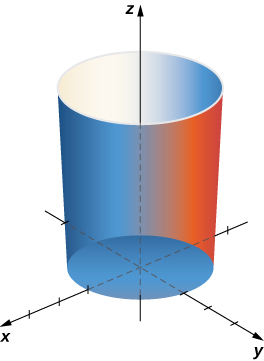
Reuse the cylinder parameterization from Example 1, compute \({\text{t}}_u\times{\text{t}}_v\) and its magnitude, then substitute into the scalar surface integral formula.
To calculate the surface integral, we first need a parameterization of the cylinder. Following Example 1, a parameterization is
\[\text{r}(u,v)=\langle 2\text{cos}\,u,2\text{sin}\,u,v\rangle ,0\le u\le 2\pi ,0\le v\le 3.\]
The tangent vectors are \({\text{t}}_{u}=\langle -2\text{sin}\,u,2\text{cos}\,u,0\rangle\) and \({\text{t}}_{v}=\langle 0,0,1\rangle .\) Then,
\[{\text{t}}_{u}\,\times \,{\text{t}}_{v}=|\begin{array}{lll}\text{i} & \text{j} & \text{k} \\ -2\text{sin}\,u & 2\text{cos}\,u & 0 \\ 0 & 0 & 1\end{array}|=⟨2\text{cos}\,u,2\text{sin}\,u,0⟩\]
and \(\Vert {\text{t}}_{u}\,\times \,{\text{t}}_{v}\Vert =\sqrt{{4\text{cos}}^{2}u+{4\text{sin}}^{2}u}=2.\) By Equation 37,
\[\begin{array}{l}\, \\ \, \\ \, \\ \,{∬}_{S}f(x,y,z)dS={∬}_{D}f(\text{r}(u,v))\Vert {\text{t}}_{u}\,\times \,{\text{t}}_{v}\Vert \,dA \\ ={∫}_{0}^{3}{∫}_{0}^{2\pi }(2\text{cos}\,u+4{\text{sin}}^{2}u)2dudv \\ =2{∫}_{0}^{3}{[2\text{sin}\,u+2u-sin(2u)]}_{0}^{2\pi }dv=2{∫}_{0}^{3}4\pi dv=24\pi .\end{array}\]
Calculate \({∬}_{S}({x}^{2}-z)dS,\) where S is the surface with parameterization \(\text{r}(u,v)=\langle v,{u}^{2}+{v}^{2},1\rangle ,0\le u\le 2,0\le v\le 3.\)
24
Calculate surface integral \({∬}_{S}f(x,y,z)dS,\) where \(f(x,y,z)={z}^{2}\) and S is the surface that consists of the piece of sphere \({x}^{2}+{y}^{2}+{z}^{2}=4\) that lies on or above plane \(z=1\) and the disk that is enclosed by intersection plane \(z=1\) and the given sphere (Figure 16).
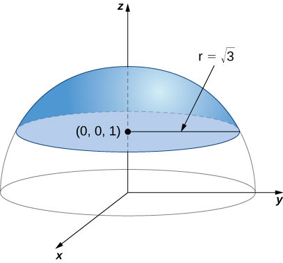
Since S is only piecewise smooth, split it into the flat disk and the spherical cap, parameterize each separately, and add the two resulting integrals.
Notice that S is not smooth but is piecewise smooth; S can be written as the union of its base \({S}_{1}\) and its spherical top \({S}_{2},\) and both \({S}_{1}\) and \({S}_{2}\) are smooth. Therefore, to calculate \({∬}_{S}{z}^{2}dS,\) we write this integral as \({∬}_{{S}_{1}}{z}^{2}dS+{∬}_{{S}_{2}}{z}^{2}dS\) and we calculate integrals \({∬}_{{S}_{1}}{z}^{2}dS\) and \({∬}_{{S}_{2}}{z}^{2}dS.\)
First, we calculate \({∬}_{{S}_{1}}{z}^{2}dS.\) To calculate this integral we need a parameterization of \({S}_{1}.\) This surface is a disk in plane \(z=1\) centered at \((0,0,1).\) To parameterize this disk, we need to know its radius. Since the disk is formed where plane \(z=1\) intersects sphere \({x}^{2}+{y}^{2}+{z}^{2}=4,\) we can substitute \(z=1\) into equation \({x}^{2}+{y}^{2}+{z}^{2}=4\text{:}\)
\[{x}^{2}+{y}^{2}+1=4⇒{x}^{2}+{y}^{2}=3.\]
Therefore, the radius of the disk is \(\sqrt{3}\) and a parameterization of \({S}_{1}\) is \(\text{r}(u,v)=\langle u\,\text{cos}\,v,u\,\text{sin}\,v,1\rangle ,0\le u\le \sqrt{3},0\le v\le 2\pi .\) The tangent vectors are \({\text{t}}_{u}=\langle \text{cos}\,v,\text{sin}\,v,0\rangle\) and \({\text{t}}_{v}=\langle \text{-}u\,\text{sin}\,v,ucosv,0\rangle ,\) and thus
\[{\text{t}}_{u}\,\times \,{\text{t}}_{v}=|\begin{array}{lll}\text{i} & \text{j} & \text{k} \\ \text{cos}\,v & \text{sin}\,v & 0 \\ \text{-}u\,\text{sin}\,v & u\,\text{cos}\,v & 0\end{array}|=\langle 0,0,u\,{\text{cos}}^{2}v+u\,{\text{sin}}^{2}v\rangle =\langle 0,0,u\rangle .\]
The magnitude of this vector is u. Therefore,
\[\begin{array}{ll}{∬}_{{S}_{1}}{z}^{2}dS & ={∫}_{0}^{\sqrt{3}}{∫}_{0}^{2\pi }f(\text{r}(u,v))\Vert {\text{t}}_{u}\,\times \,{\text{t}}_{v}\Vert \,dv\,du \\ & ={∫}_{0}^{\sqrt{3}}{∫}_{0}^{2\pi }u\,dv\,du \\ & =2\pi {∫}_{0}^{\sqrt{3}}udu \\ & =3\pi .\end{array}\]
Now we calculate \({∬}_{{S}_{2}}dS.\) To calculate this integral, we need a parameterization of \({S}_{2}.\) The parameterization of full sphere \({x}^{2}+{y}^{2}+{z}^{2}=4\) is
\[\text{r}(ϕ,θ)=\langle 2\,\text{cos}\,θ\,\text{sin}\,ϕ,2\,\text{sin}\,θ\,\text{sin}\,ϕ,2\,\text{cos}\,ϕ\rangle ,0\le θ\le 2\pi ,0\le ϕ\le \pi .\]
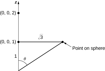
Since we are only taking the piece of the sphere on or above plane \(z=1,\) we have to restrict the domain of \(ϕ.\) To see how far this angle sweeps, notice that the angle can be located in a right triangle, as shown in Figure 17 (the \(\sqrt{3}\) comes from the fact that the base of S is a disk with radius \(\sqrt{3}).\) Therefore, the tangent of \(ϕ\) is \(\sqrt{3},\) which implies that \(ϕ\) is \(\pi \text{/}3.\) We now have a parameterization of \({S}_{2}\text{:}\)
\[\text{r}(ϕ,θ)=\langle 2\,\text{cos}\,θ\,\text{sin}\,ϕ,2\,\text{sin}\,θ\,\text{sin}\,ϕ,2\,\text{cos}\,ϕ\rangle ,0\le θ\le 2\pi ,0\le ϕ\le \pi \text{/}3.\]
The tangent vectors are
\[{\text{t}}_{ϕ}=\langle 2\,\text{cos}\,θ\,\text{cos}\,ϕ,2\,\text{sin}\,θ\,\text{cos}\,ϕ,-2\,\text{sin}\,ϕ\rangle \,\text{and}\,{\text{t}}_{θ}=\langle -2\,\text{sin}\,θ\,\text{sin}\,ϕ,u\,\text{cos}\,θ\,\text{sin}\,ϕ,0\rangle ,\]
and thus
\[\begin{array}{ll}{\text{t}}_{ϕ}\,\times \,{\text{t}}_{θ} & =|\begin{array}{lll}\text{i} & \text{j} & \text{k} \\ 2\,\text{cos}\,θ\,\text{cos}\,ϕ & 2\,\text{sin}\,θ\,\text{cos}\,ϕ & -2\,\text{sin}\,ϕ \\ -2\,\text{sin}\,θ\,\text{sin}\,ϕ & 2\,\text{cos}\,θ\,\text{sin}\,ϕ & 0\end{array}| \\ & =\langle 4\,\text{cos}\,θ\,{\text{sin}}^{2}ϕ,4\,\text{sin}\,θ\,{\text{sin}}^{2}ϕ,4\,{\text{cos}}^{2}θ\,\text{cos}\,ϕ\,\text{sin}\,ϕ+4\,{\text{sin}}^{2}θ\,\text{cos}\,ϕ\,\text{sin}\,ϕ\rangle \\ & =\langle 4\,\text{cos}\,θ\,{\text{sin}}^{2}ϕ,4\,\text{sin}\,θ\,{\text{sin}}^{2}ϕ,4\,\text{cos}\,ϕ\,\text{sin}\,ϕ\rangle .\end{array}\]
The magnitude of this vector is
\[\begin{array}{ll}\Vert {\text{t}}_{ϕ}\,\times \,{\text{t}}_{θ}\Vert & =\sqrt{16\,{\text{cos}}^{2}θ\,{\text{sin}}^{4}ϕ+16\,{\text{sin}}^{2}θ\,{\text{sin}}^{4}ϕ+16\,{\text{cos}}^{2}ϕ\,{\text{sin}}^{2}ϕ} \\ & =4\sqrt{{\text{sin}}^{4}ϕ+{\text{cos}}^{2}ϕ\,{\text{sin}}^{2}ϕ}.\end{array}\]
Therefore,
\[\begin{array}{ll}{∬}_{{S}_{2}}zdS & ={∫}_{0}^{\pi \text{/3}}{∫}_{0}^{2\pi }f(\text{r}(ϕ,θ))\Vert {\text{t}}_{ϕ}\,\times \,{\text{t}}_{θ}\Vert \,dθ\,dϕ \\ & ={∫}_{0}^{\pi \text{/3}}{∫}_{0}^{2\pi }16\,{\text{cos}}^{2}ϕ\sqrt{{\text{sin}}^{4}ϕ+{\text{cos}}^{2}ϕ\,{\text{sin}}^{2}ϕ}dθ\,dϕ \\ & =32\pi {∫}_{0}^{\pi \text{/3}}{\text{cos}}^{2}ϕ\sqrt{{\text{sin}}^{4}ϕ+{\text{cos}}^{2}ϕ\,{\text{sin}}^{2}ϕ}\,dϕ \\ & =32\pi {∫}_{0}^{\pi \text{/3}}{\text{cos}}^{2}ϕ\,\text{sin}\,ϕ\sqrt{{\text{sin}}^{2}ϕ+{\text{cos}}^{2}ϕ}\,dϕ \\ & =32\pi {∫}_{0}^{\pi \text{/3}}{\text{cos}}^{2}ϕ\,\text{sin}\,ϕ\,dϕ \\ & =32\pi {[-\frac{{\text{cos}}^{3}ϕ}{3}]}_{0}^{\pi \text{/}3}=32\pi [\frac{1}{3}-\frac{\sqrt{3}}{8}]=\frac{28\pi }{3}.\end{array}\]
Since \({∬}_{S}{z}^{2}dS={∬}_{{S}_{1}}{z}^{2}dS+{∬}_{{S}_{2}}{z}^{2}dS=3\pi +\frac{28\pi }{3}=\frac{37\pi }{3}\)
In this example we broke a surface integral over a piecewise surface into the addition of surface integrals over smooth subsurfaces. There were only two smooth subsurfaces in this example, but this technique extends to finitely many smooth subsurfaces.
Calculate surface integral \({∬}_{S}(x-y)dS,\) where S is cylinder \({x}^{2}+{y}^{2}=1,0\le z\le 2,\) including the circular top and bottom.
0
Scalar surface integrals have several real-world applications. Recall that scalar line integrals can be used to compute the mass of a wire given its density function. In a similar fashion, we can use scalar surface integrals to compute the mass of a sheet given its density function. If a thin sheet of metal has the shape of surface S and the density of the sheet at point \((x,y,z)\) is \(ρ(x,y,z),\) then mass m of the sheet is \(m={∬}_{S}ρ(x,y,z)dS.\)
A flat sheet of metal has the shape of surface \(z=1+x+2y\) that lies above rectangle \(0\le x\le 4\) and \(0\le y\le 2.\) If the density of the sheet is given by \(ρ(x,y,z)={x}^{2}yz,\) what is the mass of the sheet?
Parameterize the surface as \(\text{r}(x,y)=\langle x,y,f(x,y)\rangle\), compute \({\text{t}}_x\times{\text{t}}_y\) and its magnitude, then integrate density times that magnitude.
Let S be the surface that describes the sheet. Then, the mass of the sheet is given by \(m={∬}_{S}{x}^{2}yzdS.\) To compute this surface integral, we first need a parameterization of S. Since S is given by the function \(f(x,y)=1+x+2y,\) a parameterization of S is \(\text{r}(x,y)=\langle x,y,1+x+2y\rangle ,0\le x\le 4,0\le y\le 2.\)
The tangent vectors are \({\text{t}}_{x}=\langle 1,0,1\rangle\) and \({\text{t}}_{y}=\langle 1,0,2\rangle .\) Therefore, \({\text{t}}_{x}\,\times \,{\text{t}}_{y}=\langle -1,-2,1\rangle\) and \(\Vert {\text{t}}_{x}\,\times \,{\text{t}}_{y}\Vert =\sqrt{6}.\) By (see original),
\[\begin{array}{ll}m & ={∬}_{S}{x}^{2}yzdS \\ & =\sqrt{6}{∫}_{0}^{4}{∫}_{0}^{2}{x}^{2}y(1+x+2y)dydx \\ & =\sqrt{6}{∫}_{0}^{4}\frac{22{x}^{2}}{3}+2{x}^{3}dx \\ & =\frac{2560\sqrt{6}}{9} \\ & \approx 696.74.\end{array}\]
A piece of metal has a shape that is modeled by paraboloid \(z={x}^{2}+{y}^{2},0\le z\le 4,\) and the density of the metal is given by \(ρ(x,y,z)=z+1.\) Find the mass of the piece of metal.
\(38.401\pi \approx 120.640\)
Orientation of a Surface
Recall that when we defined a scalar line integral, we did not need to worry about an orientation of the curve of integration. The same was true for scalar surface integrals: we did not need to worry about an “orientation” of the surface of integration.
On the other hand, when we defined vector line integrals, the curve of integration needed an orientation. That is, we needed the notion of an oriented curve to define a vector line integral without ambiguity. Similarly, when we define a surface integral of a vector field, we need the notion of an oriented surface. An oriented surface is given an “upward” or “downward” orientation or, in the case of surfaces such as a sphere or cylinder, an “outward” or “inward” orientation.
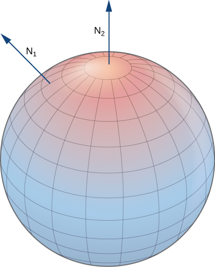
Let S be a smooth surface. For any point \((x,y,z)\) on S, we can identify two unit normal vectors \(\text{N}\) and \(\text{-}\text{N}.\) If it is possible to choose a unit normal vector N at every point \((x,y,z)\) on S so that N varies continuously over S, then S is “orientable.” Such a choice of unit normal vector at each point gives the orientation of a surface S. If you think of the normal field as describing water flow, then the side of the surface that water flows toward is the “negative” side and the side of the surface at which the water flows away is the “positive” side. Informally, a choice of orientation gives S an “outer” side and an “inner” side (or an “upward” side and a “downward” side), just as a choice of orientation of a curve gives the curve “forward” and “backward” directions.
Closed surfaces such as spheres are orientable: if we choose the outward normal vector at each point on the surface of the sphere, then the unit normal vectors vary continuously. This is called the positive orientation of the closed surface (Figure 18). We also could choose the inward normal vector at each point to give an “inward” orientation, which is the negative orientation of the surface.
A portion of the graph of any smooth function \(z=f(x,y)\) is also orientable. If we choose the unit normal vector that points “above” the surface at each point, then the unit normal vectors vary continuously over the surface. We could also choose the unit normal vector that points “below” the surface at each point. To get such an orientation, we parameterize the graph of \(f\) in the standard way: \(\text{r}(x,y)=\langle x,y,f(x,y)\rangle ,\) where x and y vary over the domain of \(f.\) Then, \({\text{t}}_{x}=\langle 1,0,{f}_{x}\rangle\) and \({\text{t}}_{y}=\langle 0,1,{f}_{y}\rangle ,\) and therefore the cross product \({\text{t}}_{x}\,\times \,{\text{t}}_{y}\) (which is normal to the surface at any point on the surface) is \(\langle \text{-}{f}_{x},\text{-}{f}_{y},1\rangle .\) Since the z component of this vector is one, the corresponding unit normal vector points “upward,” and the upward side of the surface is chosen to be the “positive” side.
Let S be a smooth orientable surface with parameterization \(\text{r}(u,v).\) For each point \(\text{r}(a,b)\) on the surface, vectors \({\text{t}}_{u}\) and \({\text{t}}_{v}\) lie in the tangent plane at that point. Vector \({\text{t}}_{u}\,\times \,{\text{t}}_{v}\) is normal to the tangent plane at \(\text{r}(a,b)\) and is therefore normal to S at that point. Therefore, the choice of unit normal vector
\[\text{N}=\frac{{\text{t}}_{u}\,\times \,{\text{t}}_{v}}{\Vert {\text{t}}_{u}\,\times \,{\text{t}}_{v}\Vert }\]
gives an orientation of surface S.
Give an orientation of cylinder \({x}^{2}+{y}^{2}={r}^{2},0\le z\le h.\)
Compute \({\text{t}}_u\times{\text{t}}_v\) for the standard cylinder parameterization, then normalize it to get N.
This surface has parameterization
\[\text{r}(u,v)=\langle r\,\text{cos}\,u,r\,\text{sin}\,u,v\rangle ,0\le u<2\pi ,0\le v\le h.\]
The tangent vectors are \({\text{t}}_{u}=\langle \text{-}r\,\text{sin}\,u,r\,\text{cos}\,u,0\rangle\) and \({\text{t}}_{v}=\langle 0,0,1\rangle .\) To get an orientation of the surface, we compute the unit normal vector
\[\text{N}=\frac{{\text{t}}_{u}\,\times \,{\text{t}}_{v}}{\Vert {\text{t}}_{u}\,\times \,{\text{t}}_{v}\Vert }.\]
In this case, \({\text{t}}_{u}\,\times \,{\text{t}}_{v}=\langle r\,\text{cos}\,u,r\,\text{sin}\,u,0\rangle\) and therefore
\[\Vert {\text{t}}_{u}\,\times \,{\text{t}}_{v}\Vert =\sqrt{{r}^{2}{\text{cos}}^{2}u+{r}^{2}{\text{sin}}^{2}u}=r.\]
An orientation of the cylinder is
\[\text{N}(u,v)=\frac{\langle r\,\text{cos}\,u,r\,\text{sin}\,u,0\rangle }{r}=\langle \text{cos}\,u,\text{sin}\,u,0\rangle .\]
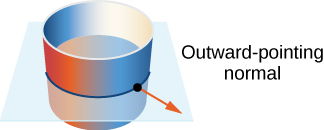
Notice that all vectors are parallel to the xy-plane, which should be the case with vectors that are normal to the cylinder. Furthermore, all the vectors point outward, and therefore this is an outward orientation of the cylinder (Figure 19).
Give the “upward” orientation of the graph of \(f(x,y)=xy.\)
\(\text{N}(x,y)=\langle \frac{\text{-}y}{\sqrt{1+{x}^{2}+{y}^{2}}},\frac{\text{-}x}{\sqrt{1+{x}^{2}+{y}^{2}}},\frac{1}{\sqrt{1+{x}^{2}+{y}^{2}}}\rangle\)
Since every curve has a “forward” and “backward” direction (or, in the case of a closed curve, a clockwise and counterclockwise direction), it is possible to give an orientation to any curve. Hence, it is possible to think of every curve as an oriented curve. This is not the case with surfaces, however. Some surfaces cannot be oriented; such surfaces are called nonorientable. Essentially, a surface can be oriented if the surface has an “inner” side and an “outer” side, or an “upward” side and a “downward” side. Some surfaces are twisted in such a fashion that there is no well-defined notion of an “inner” or “outer” side.
The classic example of a nonorientable surface is the Möbius strip. To create a Möbius strip, take a rectangular strip of paper, give the piece of paper a half-twist, and the glue the ends together (Figure 20). Because of the half-twist in the strip, the surface has no “outer” side or “inner” side. If you imagine placing a normal vector at a point on the strip and having the vector travel all the way around the band, then (because of the half-twist) the vector points in the opposite direction when it gets back to its original position. Therefore, the strip really only has one side.

Since some surfaces are nonorientable, it is not possible to define a vector surface integral on all piecewise smooth surfaces. This is in contrast to vector line integrals, which can be defined on any piecewise smooth curve.
Surface Integral of a Vector Field
With the idea of orientable surfaces in place, we are now ready to define a surface integral of a vector field. The definition is analogous to the definition of the flux of a vector field along a plane curve. Recall that if F is a two-dimensional vector field and C is a plane curve, then the definition of the flux of F along C involved chopping C into small pieces, choosing a point inside each piece, and calculating \(\text{F}·\text{N}\) at the point (where N is the unit normal vector at the point). The definition of a surface integral of a vector field proceeds in the same fashion, except now we chop surface S into small pieces, choose a point in the small (two-dimensional) piece, and calculate \(\text{F}·\text{N}\) at the point.
To place this definition in a real-world setting, let S be an oriented surface with unit normal vector N. Let v be a velocity field of a fluid flowing through S, and suppose the fluid has density \(ρ(x,y,z).\) Imagine the fluid flows through S, but S is completely permeable so that it does not impede the fluid flow (Figure 21). The mass flux of the fluid is the rate of mass flow per unit area. The mass flux is measured in mass per unit time per unit area. How could we calculate the mass flux of the fluid across S?
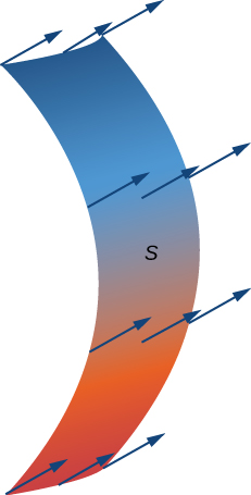
The rate of flow, measured in mass per unit time per unit area, is \(ρ\text{N}.\) To calculate the mass flux across S, chop S into small pieces \({S}_{ij}.\) If \({S}_{ij}\) is small enough, then it can be approximated by a tangent plane at some point P in \({S}_{ij}.\) Therefore, the unit normal vector at P can be used to approximate \(\text{N}(x,y,z)\) across the entire piece \({S}_{ij},\) because the normal vector to a plane does not change as we move across the plane. The component of the vector \(ρ\text{v}\) at P in the direction of N is \(ρ\text{v}·\text{N}\) at P. Since \({S}_{ij}\) is small, the dot product \(ρ\text{v}·\text{N}\) changes very little as we vary across \({S}_{ij},\) and therefore \(ρ\text{v}·\text{N}\) can be taken as approximately constant across \({S}_{ij}.\) To approximate the mass of fluid per unit time flowing across \({S}_{ij}\) (and not just locally at point P), we need to multiply \((ρ\text{v}·\text{N})(P)\) by the area of \({S}_{ij}.\) Therefore, the mass of fluid per unit time flowing across \({S}_{ij}\) in the direction of N can be approximated by \((ρ\text{v}·\text{N})\Delta {S}_{ij},\) where N, \(ρ,\) and v are all evaluated at P (Figure 22). This is analogous to the flux of two-dimensional vector field F across plane curve C, in which we approximated flux across a small piece of C with the expression \((\text{F}·\text{N})\Delta s.\) To approximate the mass flux across S, form the sum \(\sum_{i=1}^{m}\sum_{j=1}^{n}(ρ\text{v}·\text{N})\Delta {\text{S}}_{ij}.\) As pieces \({S}_{ij}\) get smaller, the sum \(\sum_{i=1}^{m}\sum_{j=1}^{n}(ρ\text{v}·\text{N})\Delta {\text{S}}_{ij}\) gets arbitrarily close to the mass flux. Therefore, the mass flux is
\[{∬}_{s}ρ\text{v}·\text{N}dS=\underset{m,n\to \infty }{\text{lim}}\sum_{i=1}^{m}\sum_{j=1}^{n}(ρ\text{v}·\text{N})\Delta {\text{S}}_{ij}.\]
This is a surface integral of a vector field. Letting the vector field \(ρ\text{v}\) be an arbitrary vector field F leads to the following definition.
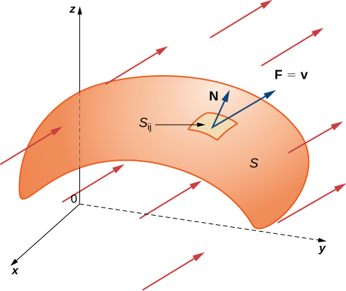
Let F be a continuous vector field with a domain that contains oriented surface S with unit normal vector N. The surface integral of F over S is
\[{∬}_{S}\text{F}·d\text{S}={∬}_{S}\text{F}·\text{N}dS.\]
Notice the parallel between this definition and the definition of vector line integral \({∫}_{C}\text{F}·\text{N}ds.\) A surface integral of a vector field is defined in a similar way to a flux line integral across a curve, except the domain of integration is a surface (a two-dimensional object) rather than a curve (a one-dimensional object). Integral \({∬}_{S}\text{F}·\text{N}dS\) is called the flux of F across S, just as integral \({∫}_{C}\text{F}·\text{N}ds\) is the flux of F across curve C. A surface integral over a vector field is also called a flux integral.
Just as with vector line integrals, surface integral \({∬}_{S}\text{F}·\text{N}dS\) is easier to compute after surface S has been parameterized. Let \(\text{r}(u,v)\) be a parameterization of S with parameter domain D. Then, the unit normal vector is given by \(\text{N}=\frac{{\text{t}}_{u}\,\times \,{\text{t}}_{v}}{\Vert {\text{t}}_{u}\,\times \,{\text{t}}_{v}\Vert }\) and, from Equation 61, we have
\[\begin{array}{ll}{∬}_{S}\text{F}·d\text{S} & ={∬}_{S}\text{F}·\text{N}dS \\ & ={∬}_{S}\text{F}·\frac{{\text{t}}_{u}\,\times \,{\text{t}}_{v}}{\Vert {\text{t}}_{u}\,\times \,{\text{t}}_{v}\Vert }dS \\ & ={∬}_{D}(\text{F}(\text{r}(u,v))·\frac{{\text{t}}_{u}\,\times \,{\text{t}}_{v}}{\Vert {\text{t}}_{u}\,\times \,{\text{t}}_{v}\Vert })\Vert {\text{t}}_{u}\,\times \,{\text{t}}_{v}\Vert dA \\ & ={∬}_{D}(\text{F}(\text{r}(u,v))·({\text{t}}_{u}\,\times \,{\text{t}}_{v}))dA.\end{array}\]
Therefore, to compute a surface integral over a vector field we can use the equation
\[{∬}_{S}\text{F}·\text{N}dS={∬}_{D}(\text{F}(\text{r}(u,v))·({\text{t}}_{u}\,\times \,{\text{t}}_{v}))dA.\]
Calculate the surface integral \({∬}_{S}\text{F}·\text{N}dS,\) where \(\text{F}=\langle \text{-}y,x,0\rangle\) and \(S\) is the surface with parameterization \(\text{r}(u,v)=\langle u,{v}^{2}-u,u+v\rangle ,0\le u<3,0\le v\le 4.\)
Compute \({\text{t}}_u\times{\text{t}}_v\) (no need to normalize), dot it with \(\text{F}(\text{r}(u,v))\), and integrate over the rectangular parameter domain.
The tangent vectors are \({\text{t}}_{u}=\langle 1,-1,1\rangle\) and \({\text{t}}_{v}=\langle 0,2v,1\rangle .\) Therefore,
\[{\text{t}}_{u}\,\times \,{\text{t}}_{v}=\langle -1-2v,-1,2v\rangle .\]
By Equation 63,
\[\begin{array}{ll}{∬}_{S}\text{F}·d\text{S} & ={∫}_{0}^{4}{∫}_{0}^{3}\text{F}(\text{r}(u,v))·({\text{t}}_{u}\,\times \,{\text{t}}_{v})dudv \\ & ={∫}_{0}^{4}{∫}_{0}^{3}\langle u-{v}^{2},u,0\rangle ·\langle -1-2v,-1,2v\rangle \,dudv \\ & ={∫}_{0}^{4}{∫}_{0}^{3}[(u-{v}^{2})(-1-2v)-u]dudv \\ & ={∫}_{0}^{4}{∫}_{0}^{3}(2{v}^{3}+{v}^{2}-2uv-2u)dudv \\ & ={{∫}_{0}^{4}[2{v}^{3}u+{v}^{2}u-v{u}^{2}-{u}^{2}]}_{0}^{3}dv \\ & ={∫}_{0}^{4}(6{v}^{3}+3{v}^{2}-9v-9)dv \\ & ={[\frac{3{v}^{4}}{2}+{v}^{3}-\frac{9{v}^{2}}{2}-9v]}_{0}^{4} \\ & =340.\end{array}\]
Therefore, the flux of F across S is 340.
Calculate surface integral \({∬}_{S}\text{F}·d\text{S},\) where \(\text{F}=\langle 0,\text{-}z,y\rangle\) and S is the portion of the unit sphere in the first octant with outward orientation.
0
Let \(\text{v}(x,y,z)=\langle 2x,2y,z\rangle\) represent a velocity field (with units of meters per second) of a fluid with constant density 80 kg/m3. Let S be hemisphere \({x}^{2}+{y}^{2}+{z}^{2}=9\) with \(z\ge 0\) such that S is oriented outward. Find the mass flow rate of the fluid across S.
Parameterize the hemisphere, compute \({\text{t}}_{\phi}\times{\text{t}}_{\theta}\) and confirm it points outward, then dot with \(\rho\text{v}\) and integrate.
A parameterization of the surface is
\[\text{r}(ϕ,θ)=\langle 3\,\text{cos}\,θ\,\text{sin}\,ϕ,3\,\text{sin}\,θ\,\text{sin}\,ϕ,3\,\text{cos}\,ϕ\rangle ,0\le θ\le 2\pi ,0\le ϕ\le \pi \text{/}2.\]
As in Example 7, the tangent vectors are
\[{\text{t}}_{θ}=\langle -3\,\text{sin}\,θ\,\text{sin}\,ϕ,3\,\text{cos}\,θ\,\text{sin}\,ϕ,0\rangle \,\text{and}\,{\text{t}}_{ϕ}=\langle 3\,\text{cos}\,θ\,\text{cos}\,ϕ,3\,\text{sin}\,θ\,\text{cos}\,ϕ,-3\,\text{sin}\,ϕ\rangle ,\]
and their cross product is
\[{\text{t}}_{ϕ}\,\times \,{\text{t}}_{θ}=\langle 9\,\text{cos}\,θ\,{\text{sin}}^{2}ϕ,9\,\text{sin}\,θ\,{\text{sin}}^{2}ϕ,9\,\text{sin}\,ϕ\,\text{cos}\,ϕ\rangle .\]
Notice that each component of the cross product is positive, and therefore this vector gives the outward orientation. Therefore we use the orientation \(\text{N}=\langle 9\,\text{cos}\,θ\,{\text{sin}}^{2}ϕ,9\,\text{sin}\,θ\,{\text{sin}}^{2}ϕ,9\,\text{sin}\,ϕ\,\text{cos}\,ϕ\rangle\) for the sphere.
By Equation 62,
\[\begin{array}{ll}{∬}_{S}ρ\text{v}·d\text{S} & =80{∫}_{0}^{2\pi }{∫}_{0}^{\pi \text{/}2}\text{v}(\text{r}(ϕ,θ))·({\text{t}}_{ϕ}\,\times \,{\text{t}}_{θ})dϕdθ \\ & =80{∫}_{0}^{2\pi }{∫}_{0}^{\pi \text{/}2} \\ & =80{∫}_{0}^{2\pi }{∫}_{0}^{\pi \text{/}2}\begin{array}{l}\langle 6\,\text{cos}\,θ\,\text{sin}\,ϕ,6\,\text{sin}\,θ\,\text{sin}\,ϕ,3\,\text{cos}\,ϕ\rangle \\ ·\langle 9\,\text{cos}\,θ\,{\text{sin}}^{2}ϕ,9\,\text{sin}\,θ\,{\text{sin}}^{2}ϕ,9\,\text{sin}\,ϕ\,\text{cos}\,ϕ\rangle dϕdθ\end{array} \\ & =80{∫}_{0}^{2\pi }{∫}_{0}^{\pi \text{/}2}54\,{\text{sin}}^{3}ϕ+27\,{\text{cos}}^{2}ϕ\,\text{sin}\,ϕdϕdθ \\ & =80{∫}_{0}^{2\pi }{∫}_{0}^{\pi \text{/}2}54(1-{\text{cos}}^{2}ϕ)\text{sin}\,ϕ+27\,{\text{cos}}^{2}ϕ\,\text{sin}\,ϕdϕdθ \\ & =80{∫}_{0}^{2\pi }{∫}_{0}^{\pi \text{/}2}54\,\text{sin}\,ϕ-27\,{\text{cos}}^{2}ϕ\,\text{sin}\,ϕdϕdθ \\ & =80{∫}_{0}^{2\pi }{[-54\,\text{cos}\,ϕ+9\,{\text{cos}}^{3}ϕ]}_{ϕ=0}^{ϕ=2\pi }dθ \\ & =80{∫}_{0}^{2\pi }45dθ=7200\pi .\end{array}\]
Therefore, the mass flow rate is \(7200\pi \,\text{kg}\text{/}\text{sec}\text{/}{\text{m}}^{2}.\)
Let \(\text{v}(x,y,z)=\langle {x}^{2}+{y}^{2},z,4y\rangle\) m/sec represent a velocity field of a fluid with constant density 100 kg/m3. Let S be the half-cylinder \(\text{r}(u,v)=\langle \text{cos}\,u,\text{sin}\,u,v\rangle ,0\le u\le \pi ,0\le v\le 2\) oriented outward. Calculate the mass flux of the fluid across S.
400 kg/sec/m
In Example 14, we computed the mass flux, which is the rate of mass flow per unit area. If we want to find the flow rate (measured in volume per time) instead, we can use flux integral \({∬}_{S}\text{v}·\text{N}dS,\) which leaves out the density. Since the flow rate of a fluid is measured in volume per unit time, flow rate does not take mass into account. Therefore, we have the following characterization of the flow rate of a fluid with velocity v across a surface S:
\[\text{Flow rate of fluid across}\,S={∬}_{S}v·d\text{S}.\]
To compute the flow rate of the fluid in Example 14, we simply remove the density constant, which gives a flow rate of \(90\pi {\,\text{m}}^{3}\text{/}\text{sec}.\)
Both mass flux and flow rate are important in physics and engineering. Mass flux measures how much mass is flowing across a surface; flow rate measures how much volume of fluid is flowing across a surface.
In addition to modeling fluid flow, surface integrals can be used to model heat flow. Suppose that the temperature at point \((x,y,z)\) in an object is \(T(x,y,z).\) Then the heat flow is a vector field proportional to the negative temperature gradient in the object. To be precise, the heat flow is defined as vector field \(\text{F}=\text{-}k∇T,\) where the constant k is the thermal conductivity of the substance from which the object is made (this constant is determined experimentally). The rate of heat flow across surface S in the object is given by the flux integral
\[{∬}_{S}\text{F}·d\text{S}={∬}_{S}\text{-}k∇T·d\text{S}.\]
A cast-iron solid cylinder is given by inequalities \({x}^{2}+{y}^{2}\le 1,\) \(1\le z\le 4.\) The temperature at point \((x,y,z)\) in a region containing the cylinder is \(T(x,y,z)=({x}^{2}+{y}^{2})z.\) Given that the thermal conductivity of cast iron is 55, find the heat flow across the boundary of the solid if this boundary is oriented outward.
Split the boundary into its three smooth pieces (bottom disk, top disk, cylindrical side), parameterize each, and add the flux of \(-k\nabla T\) across all three.
Let S denote the boundary of the object. To find the heat flow, we need to calculate flux integral \({∬}_{S}\text{-}k∇T·d\text{S}.\) Notice that S is not a smooth surface but is piecewise smooth, since S is the union of three smooth surfaces (the circular top and bottom, and the cylindrical side). Therefore, we calculate three separate integrals, one for each smooth piece of S. Before calculating any integrals, note that the gradient of the temperature is \(∇T=\langle 2xz,2yz,{x}^{2}+{y}^{2}\rangle .\)
First we consider the circular bottom of the object, which we denote \({S}_{1}.\) We can see that \({S}_{1}\) is a circle of radius 1 centered at point \((0,0,1),\) sitting in plane \(z=1.\) This surface has parameterization \(\text{r}(u,v)=\langle v\,\text{cos}\,u,v\,\text{sin}\,u,1\rangle ,0\le u<2\pi ,0\le v\le 1.\) Therefore,
\[{\text{t}}_{u}=\langle \text{-}v\,\text{sin}\,u,v\,\text{cos}\,u,0\rangle \,\text{and}\,{\text{t}}_{v}=\langle \text{cos}\,u,v\,\text{sin}\,u,0\rangle ,\]
and
\[{\text{t}}_{u}\,\times \,{\text{t}}_{v}=\langle 0,0,\text{-}v\,{\text{sin}}^{2}u-v\,{\text{cos}}^{2}u\rangle =\langle 0,0,\text{-}v\rangle .\]
Since the surface is oriented outward and \({S}_{1}\) is the bottom of the object, it makes sense that this vector points downward. By Equation 63, the heat flow across \({S}_{1}\) is
\[\begin{array}{ll}{∬}_{{S}_{1}}\text{-}k∇T·d\text{S} & =-55{∫}_{0}^{2\pi }{∫}_{0}^{1}∇T(u,v)·({\text{t}}_{u}\,\times \,{\text{t}}_{v})dvdu \\ & =-55{∫}_{0}^{2\pi }{∫}_{0}^{1}\langle 2v\,\text{cos}\,u,2v\,\text{sin}\,u,{v}^{2}{\text{cos}}^{2}u+{v}^{2}{\text{sin}}^{2}u\rangle ·\langle 0,0,\text{-}v\rangle dvdu \\ & =-55{∫}_{0}^{2\pi }{∫}_{0}^{1}\langle 2v\,\text{cos}\,u,2v\,\text{sin}\,u,{v}^{2}\rangle ·\langle 0,0,\text{-}v\rangle dvdu \\ & =-55{∫}_{0}^{2\pi }{∫}_{0}^{1}\text{-}{v}^{3}dvdu=-55{∫}_{0}^{2\pi }-\frac{1}{4}du=\frac{55\pi }{2}.\end{array}\]
Now let’s consider the circular top of the object, which we denote \({S}_{2}.\) We see that \({S}_{2}\) is a circle of radius 1 centered at point \((0,0,4),\) sitting in plane \(z=4.\) This surface has parameterization \(\text{r}(u,v)=\langle v\,\text{cos}\,u,v\,\text{sin}\,u,4\rangle ,0\le u<2\pi ,0\le v\le 1.\) Therefore,
\[{\text{t}}_{u}=\langle \text{-}v\,\text{sin}\,u,v\,\text{cos}\,u,0\rangle \,\text{and}\,{\text{t}}_{v}=\langle \text{cos}\,u,v\,\text{sin}\,u,0\rangle ,\]
and
\[{\text{t}}_{u}\,\times \,{\text{t}}_{v}=\langle 0,0,\text{-}v\,{\text{sin}}^{2}u-v\,{\text{cos}}^{2}u\rangle =\langle 0,0,\text{-}v\rangle .\]
Since the surface is oriented outward and \({S}_{1}\) is the top of the object, we instead take vector \({\text{t}}_{v}\,\times \,{\text{t}}_{u}=\langle 0,0,v\rangle .\) By Equation 63, the heat flow across \({S}_{1}\) is
\[\begin{array}{ll}∫{∫}_{{S}_{2}}\text{-}k∇T·d\text{S} & =-55{∫}_{0}^{2\pi }{∫}_{0}^{1}∇T(u,v)·({\text{t}}_{v}\,\times \,{\text{t}}_{u})dvdu \\ & =-55{∫}_{0}^{2\pi }{∫}_{0}^{1}\langle 8v\,\text{cos}\,u,8v\,\text{sin}\,u,{v}^{2}{\text{cos}}^{2}u+{v}^{2}{\text{sin}}^{2}u\rangle ·\langle 0,0,v\rangle dvdu \\ & =-55{∫}_{0}^{2\pi }{∫}_{0}^{1}\langle 8v\,\text{cos}\,u,8v\,\text{sin}\,u,{v}^{2}\rangle ·\langle 0,0,v\rangle dvdu \\ & =-55{∫}_{0}^{2\pi }{∫}_{0}^{1}{v}^{3}dvdu=-\frac{55\pi }{2}.\end{array}\]
Last, let’s consider the cylindrical side of the object. This surface has parameterization \(\text{r}(u,v)=\langle \text{cos}\,u,\text{sin}\,u,v\rangle ,0\le u<2\pi ,1\le v\le 4.\) By Example 9, we know that \({\text{t}}_{u}\,\times \,{\text{t}}_{v}=\langle \text{cos}\,u,\text{sin}\,u,0\rangle .\) By Equation 63,
\[\begin{array}{ll}{∬}_{{S}_{3}}\text{-}k∇T·d\text{S} & =-55{∫}_{0}^{2\pi }{∫}_{1}^{4}∇T(u,v)·({\text{t}}_{v}\,\times \,{\text{t}}_{u})dvdu \\ & =-55{∫}_{0}^{2\pi }{∫}_{1}^{4}\langle 2v\,\text{cos}\,u,2v\,\text{sin}\,u,{\text{cos}}^{2}u+{\text{sin}}^{2}u\rangle ·\langle \text{cos}\,u,\text{sin}\,u,0\rangle dvdu \\ & =-55{∫}_{0}^{2\pi }{∫}_{0}^{1}\langle 2v\,\text{cos}\,u,2v\,\text{sin}\,u,1\rangle ·\langle \text{cos}\,u,\text{sin}\,u,0\rangle dvdu \\ & =-55{∫}_{0}^{2\pi }{∫}_{0}^{1}(2v\,{\text{cos}}^{2}u+2v\,{\text{sin}}^{2}u)dvdu \\ & =-55{∫}_{0}^{2\pi }{∫}_{0}^{1}2vdvdu=-55{∫}_{0}^{2\pi }du=-110\pi .\end{array}\]
Therefore, the rate of heat flow across S is \(\frac{55\pi }{2}-\frac{55\pi }{2}-110\pi =-110\pi .\)
A cast-iron solid ball is given by inequality \({x}^{2}+{y}^{2}+{z}^{2}\le 1.\) The temperature at a point in a region containing the ball is \(T(x,y,z)=\frac{1}{3}({x}^{2}+{y}^{2}+{z}^{2}).\) Find the heat flow across the boundary of the solid if this boundary is oriented outward.
\(-\frac{440\pi }{3}\)
Key Concepts
- Surfaces can be parameterized, just as curves can be parameterized. In general, surfaces must be parameterized with two parameters. (See Example 1.)
- Surfaces can sometimes be oriented, just as curves can be oriented. Some surfaces, such as a Möbius strip, cannot be oriented. (See Example 12.)
- A surface integral is like a line integral in one higher dimension. The domain of integration of a surface integral is a surface in a plane or space, rather than a curve in a plane or space.
- The integrand of a surface integral can be a scalar function or a vector field. To calculate a surface integral with an integrand that is a function, use Equation 37. To calculate a surface integral with an integrand that is a vector field, use Equation 61. (See Example 9 and Example 13.)
- If S is a surface, then the area of S is \(∫{∫}_{S}dS.\) (See Example 6.)
Key Equations
| Scalar surface integral | \(∫{∫}_{S}f(x,y,z)dS=∫{∫}_{D}f(\text{r}(u,v))||{\text{t}}_{u}\,\times \,{\text{t}}_{v}||dA\) |
| Flux integral | \({∬}_{S}\text{F}·\text{N}dS={∬}_{S}\text{F}·d\text{S}={∬}_{D}\text{F}(\text{r}(u,v))·({\text{t}}_{u}\,\times \,{\text{t}}_{v})dA\) |
Section Exercises
For the following exercises, determine whether the statements are true or false.
If surface S is given by \(\{(x,y,z):0\le x\le 1,0\le y\le 1,z=10\},\) then \({∬}_{S}f(x,y,z)dS={∫}_{0}^{1}{∫}_{0}^{1}f(x,y,10)dxdy.\)
True
If surface S is given by \(\{(x,y,z):0\le x\le 1,0\le y\le 1,z=x\},\) then \({∬}_{S}f(x,y,z)dS={∫}_{0}^{1}{∫}_{0}^{1}f(x,y,x)dxdy.\)
Surface \(\text{r}=\langle v\,\text{cos}\,u,v\,\text{sin}\,u,{v}^{2}\rangle ,\,\text{for}\,0\le u\le \pi ,0\le v\le 2,\) is the same as surface \(\text{r}=\langle \sqrt{v}\,\text{cos}\,2u,\sqrt{v}\,\text{sin}\,2u,v\rangle ,\) for \(0\le u\le \frac{\pi }{2},0\le v\le 4.\)
True
Given the standard parameterization of a sphere, normal vectors \({\text{t}}_{u}^{}\,\times \,{\text{t}}_{v}\) are outward normal vectors.
For the following exercises, find parametric descriptions for the following surfaces.
Plane \(3x-2y+z=2\)
\(\text{r}(u,v)=\langle u,v,2-3u+2v\rangle\) for \(\text{-}\infty \le u<\infty\) and \(\text{-}\infty \le v<\infty .\)
Paraboloid \(z={x}^{2}+{y}^{2},\) for \(0\le z\le 9.\)
Plane \(2x-4y+3z=16\)
\(\text{r}(u,v)=\langle u,v,\frac{1}{3}(16-2u+4v)\rangle\) for \(|u|<\infty\) and \(|v|<\infty .\)
The frustum of cone \({z}^{2}={x}^{2}+{y}^{2},\,\text{for}\,2\le z\le 8\)
The portion of cylinder \({x}^{2}+{y}^{2}=9\) in the first octant, for \(0\le z\le 3\)
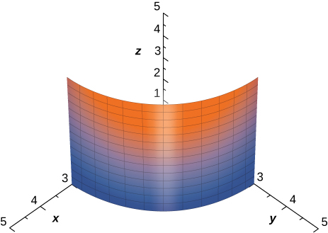
\(\text{r}(u,v)=\langle 3\,\text{cos}\,u,3\,\text{sin}\,u,v\rangle\) for \(0\le u\le \frac{\pi }{2},0\le v\le 3\)
A cone with base radius r and height h, where r and h are positive constants
For the following exercises, use a computer algebra system to approximate the area of the following surfaces using a parametric description of the surface.
[T] Half cylinder \(\{(r,θ,z):r=4,0\le θ\le \pi ,0\le z\le 7\}\)
\(A=28\pi =87.9646\)
[T] Plane \(z=10-x-y\) above square \(|x|\le 2,|y|\le 2\)
For the following exercises, let S be the hemisphere \({x}^{2}+{y}^{2}+{z}^{2}=4,\) with \(z\ge 0,\) and evaluate each surface integral.
\({∬}_{S}zdS\)
\({∬}_{S}zdS=8\pi\)
\({∬}_{S}(x-2y)dS\)
\({∬}_{S}({x}^{2}+{y}^{2})zdS\)
\({∬}_{S}({x}^{2}+{y}^{2})zdS=16\pi\)
For the following exercises, evaluate \(∫{∫}_{S}\text{F}·\text{N}dS\) for vector field F, where N is an upward pointing normal vector to surface S.
\(\text{F}(x,y,z)=x\text{i}+2y\text{j}-3z\text{k},\) and S is that part of plane \(15x-12y+3z=6\) that lies above unit square \(0\le x\le 1,0\le y\le 1.\)
\(\text{F}(x,y,z)=x\text{i}+y\text{j},\) and S is hemisphere \(z=\sqrt{1-{x}^{2}-{y}^{2}}.\)
\({∬}_{S}\text{F}·\text{N}dS=\frac{4\pi }{3}\)
\(\text{F}(x,y,z)={x}^{2}\text{i}+{y}^{2}\text{j}+{z}^{2}\text{k},\) and S is the portion of plane \(z=y+1\) that lies inside cylinder \({x}^{2}+{y}^{2}=1.\)
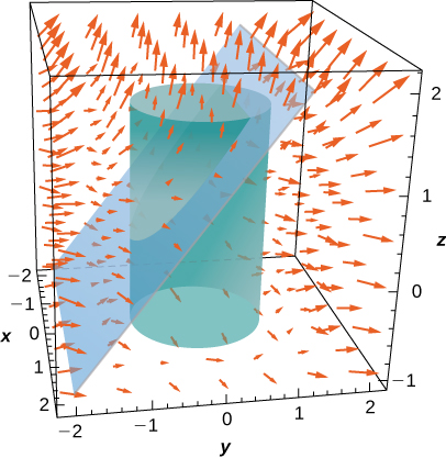
For the following exercises, approximate the mass of the lamina that has the shape of given surface S. Round to four decimal places.
[T] S is surface \(z=4-x-2y,\,\text{with}\,z\ge 0\text{,}\,x\ge 0\text{,}\,y\ge 0\text{;}\,ρ=x.\)
\(m\approx 13.0639\)
[T] S is surface \(z={x}^{2}+{y}^{2},\,\text{with}\,z\le 1\text{;}\,ρ=z.\)
[T] S is surface \({x}^{2}+{y}^{2}+{z}^{2}=5,\,\text{with}\,z\ge 1\text{;}\,ρ={θ}^{2}.\)
\(m\approx 228.5313\)
Evaluate \({∬}_{S}({y}^{2}z\text{i}+{y}^{3}\text{j}+xz\text{k})·dS\text{,}\) where S is the surface of cube \(-1\le x\le 1,-1\le y\le 1,\text{and}\,0\le z\le 2.\) Assume an outward pointing normal.
Evaluate surface integral \({∬}_{S}gdS,\) where \(g(x,y,z)=xz+2{x}^{2}-3xy\) and S is the portion of plane \(2x-3y+z=6\) that lies over unit square R: \(0\le x\le 1\text{,}\,0\le y\le 1.\)
\({∬}_{S}gdS=3\sqrt{14}\)
Evaluate \({∬}_{S}({x}^{2}+y-z)dS\text{,}\) where \(S\) is the surface defined parametrically by \(\text{r}(u,v)=(2u+v)\text{i}+(u-2v)\text{j}+(u+3v)\text{k}\) for \(0\le u\le 1,\,\text{and}\,0\le v\le 2.\)
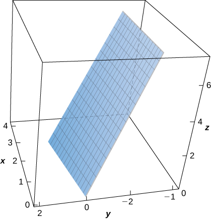
[T] Evaluate \({∬}_{S}(x-{y}^{2}+z)dS\text{,}\) where S is the surface defined by \(\text{r}(u,v)={u}^{2}\text{i}+v\text{j}+u\text{k}\text{,}\,0\le u\le 1\text{,}\,0\le v\le 1.\)
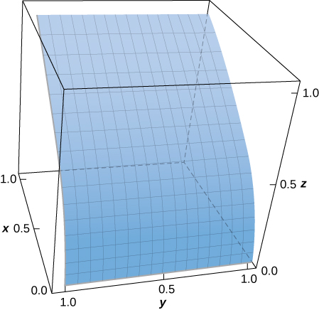
\({∬}_{S}(x-{y}^{2}+z)dS\approx 0.9617\)
[T] Evaluate \(∫{∫}_{S}({x}^{2}+{y}^{2}-z)dS\) where \(S\) is the surface defined by \(\text{r}(u,v)=u\text{i}-{u}^{2}\text{j}+v\text{k}\text{,}\,0\le u\le 2\text{,}\,0\le v\le 1.\)
Evaluate \({∬}_{S}({x}^{2}+{y}^{2})dS,\) where S is the surface of hemisphere \(z=\sqrt{1-{x}^{2}-{y}^{2}},\) and above the plane \(z=0.\)
\({∬}_{S}({x}^{2}+{y}^{2})dS=\frac{4\pi }{3}\)
Evaluate \({∬}_{S}({x}^{2}+{y}^{2}+{z}^{2})dS,\) where S is the portion of plane \(z=x+1\) that lies inside cylinder \({x}^{2}+{y}^{2}=1.\)
[T] Evaluate \({∬}_{S}{x}^{2}zdS,\) where S is the portion of cone \({z}^{2}={x}^{2}+{y}^{2}\) that lies between planes \(z=1\) and \(z=4.\)
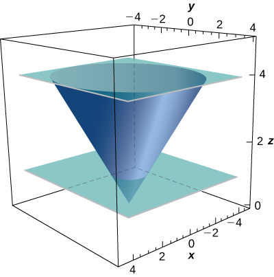
\({∬}_{S}{x}^{2}zdS=\frac{1023\pi \sqrt{2}}{5}\)
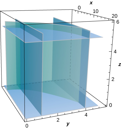
[T] Evaluate \({∬}_{S}(xz\text{/}y)dS,\) where S is the portion of cylinder \(x={y}^{2}\) that lies in the first octant between planes \(z=0,z=5,y=1,\) and \(y=4.\)
[T] Evaluate \({∬}_{S}(z+y)dS,\) where S is the part of the graph of \(z=\sqrt{1-{x}^{2}}\) in the first octant between the xz-plane and plane \(y=3.\)
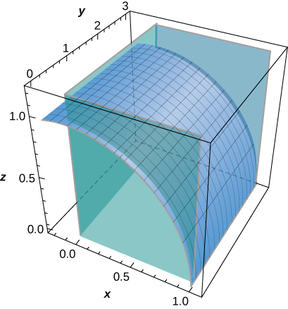
\({∬}_{S}(z+y)dS\approx 10.1\)
Evaluate \({∬}_{S}xyzdS\) if S is the part of plane \(z=x+y\) that lies over the triangular region in the xy-plane with vertices (0, 0, 0), (1, 0, 0), and (0, 2, 0).
Find the mass of a lamina of density \(ρ(x,y,z)=z\) in the shape of hemisphere \(z={({a}^{2}-{x}^{2}-{y}^{2})}^{1\text{/}2}.\)
\(m=\pi {a}^{3}\)
Compute \({∬}_{S}\text{F}·\text{N}dS,\) where \(\text{F}(x,y,z)=x\text{i}-5y\text{j}+4z\text{k}\) and N is an outward normal vector of S, where S is the union of two squares \({S}_{1}:x=0\text{,}\,0\le y\le 1\text{,}\,0\le z\le 1\) and \({S}_{2}:z=1\text{,}\,0\le x\le 1\text{,}\,0\le y\le 1.\)
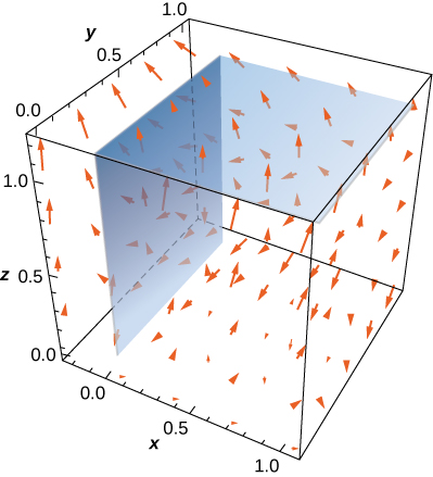
Compute \({∬}_{S}\text{F}·\text{N}dS,\) where \(\text{F}(x,y,z)=xy\text{i}+z\text{j}+(x+y)\text{k}\) and N is an upward pointing normal vector \(S\) , where S is the triangular region of the plane \(x+y+z=1\) in the first octant.
\({∬}_{S}\text{F}·\text{N}dS=\frac{13}{24}\)
Compute \({∬}_{S}\text{F}·\text{N}dS,\) where \(\text{F}(x,y,z)=2yz\text{i}+({\text{tan}}^{-1}(xz))\text{j}+{e}^{xy}\text{k}\) and N is an outward normal vector of S, where S is the surface of sphere \({x}^{2}+{y}^{2}+{z}^{2}=1.\)
Compute \({∬}_{S}\text{F}·\text{N}dS,\) where \(\text{F}(x,y,z)=xyz\text{i}+xyz\text{j}+xyz\text{k}\) and N is an outward normal vector S, where S is the surface of the five faces of the unit cube \(0\le x\le 1\text{,}\,0\le y\le 1\text{,}\,0\le z\le 1\) missing \(z=0.\)
\({∬}_{S}\text{F}·\text{N}dS=\frac{3}{4}\)
For the following exercises, express the surface integral as an iterated double integral by using a projection on S on the yz-plane.
\({∬}_{S}x{y}^{2}{z}^{3}dS;\) S is the first-octant portion of plane \(2x+3y+4z=12.\)
\({∬}_{S}({x}^{2}-2y+z)dS;\) S is the portion of the graph of \(4x+y=8\) bounded by the coordinate planes and plane \(z=6.\)
\(\int_{0}^{8}\int_{0}^{6}(4-3y+\frac{1}{16}{y}^{2}+z)(\frac{1}{4}\sqrt{17})dzdy\)
For the following exercises, express the surface integral as an iterated double integral by using a projection on S on the xz-plane
\({∬}_{S}x{y}^{2}{z}^{3}dS;\) S is the first-octant portion of plane \(2x+3y+4z=12.\)
\({∬}_{S}({x}^{2}-2y+z)dS;\) S is the portion of the graph of \(4x+y=8\) bounded by the coordinate planes and plane \(z=6.\)
\(\int_{0}^{2}\int_{0}^{6}[{x}^{2}-2(8-4x)+z]\sqrt{17}dzdx\)
Evaluate surface integral \({∬}_{S}yzdS,\) where S is the first-octant part of plane \(x+y+z=λ,\) where \(λ\) is a positive constant.
Evaluate surface integral \({∬}_{S}({x}^{2}z+{y}^{2}z)dS,\) where S is hemisphere \({x}^{2}+{y}^{2}+{z}^{2}={a}^{2},z\ge 0.\)
\({∬}_{S}({x}^{2}z+{y}^{2}z)dS=\frac{\pi {a}^{5}}{2}\)
Evaluate surface integral \({∬}_{S}zdS,\) where S is surface \(z=\sqrt{{x}^{2}+{y}^{2}},0\le z\le 2.\)
Evaluate surface integral \({∬}_{S}{x}^{2}yzdS,\) where S is the part of plane \(z=1+2x+3y\) that lies above rectangle \(0\le x\le 3\,\text{and}\,0\le y\le 2.\)
\({∬}_{S}{x}^{2}yzdS=171\sqrt{14}\)
Evaluate surface integral \({∬}_{S}yzdS,\) where S is plane \(x+y+z=1\) that lies in the first octant.
Evaluate surface integral \({∬}_{S}yzdS,\) where S is the part of plane \(z=y+3\) that lies inside cylinder \({x}^{2}+{y}^{2}=1.\)
\({∬}_{S}yzdS=\frac{\sqrt{2}\pi }{4}\)
For the following exercises, use geometric reasoning to evaluate the given surface integrals.
\({∬}_{S}\sqrt{{x}^{2}+{y}^{2}+{z}^{2}}dS,\) where S is surface \({x}^{2}+{y}^{2}+{z}^{2}=4,z\ge 0\)
\({∬}_{S}(x\text{i}+y\text{j})·dS,\) where S is surface \({x}^{2}+{y}^{2}=4,1\le z\le 3,\) oriented with unit normal vectors pointing outward
\({∬}_{S}(x\text{i}+y\text{j})·dS=16\pi\)
\({∬}_{S}(z\text{k})·dS,\) where S is disc \({x}^{2}+{y}^{2}\le 9\) on plane \(z=4,\) oriented with unit normal vectors pointing upward
A lamina has the shape of a portion of sphere \({x}^{2}+{y}^{2}+{z}^{2}={a}^{2}\) that lies within cone \(z=\sqrt{{x}^{2}+{y}^{2}}.\) Let S be the spherical shell centered at the origin with radius a, and let C be the right circular cone with a vertex at the origin and an axis of symmetry that coincides with the z-axis. Determine the mass of the lamina if \(ρ(x,y,z)={x}^{2}{y}^{2}z.\)
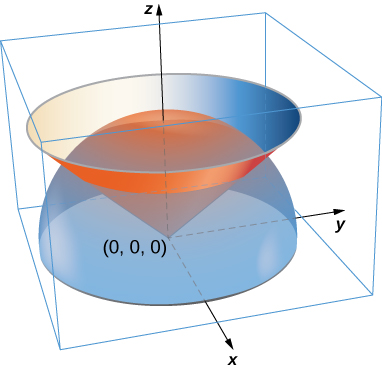
\(m=\frac{\pi {a}^{7}}{192}\)
A lamina has the shape of a portion of sphere \({x}^{2}+{y}^{2}+{z}^{2}={a}^{2}\) that lies within cone \(z=\text{cot}{φ}_{0}\sqrt{{x}^{2}+{y}^{2}}\) Let S be the spherical shell centered at the origin with radius a, and let C be the right circular cone with a vertex at the origin and an axis of symmetry that coincides with the z-axis. Suppose the angle between the sides of the cone and the z-axis is \({ϕ}_{0},\,\text{with}\,0\le {ϕ}_{0}<\frac{\pi }{2}.\) Determine the mass of that portion of the shape enclosed in the intersection of S and C. Assume \(ρ(x,y,z)={x}^{2}{y}^{2}z.\)
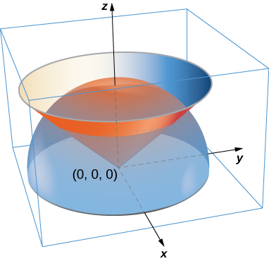
A paper cup has the shape of an inverted right circular cone of height 6 in. and radius of top 3 in. If the cup is full of water weighing \(62.5\,\text{lb}\text{/}{\text{ft}}^{3},\) find the total force exerted by the water on the inside surface of the cup.
\(F\approx 4.57\,\text{lb}.\)
For the following exercises, the heat flow vector field for conducting objects is \(\text{F}=\text{-}k∇T,\,\text{where}\,T(x,y,z)\) is the temperature in the object and \(k>0\) is a constant that depends on the material. Find the outward flux of F across the following surfaces S for the given temperature distributions and assume \(k=1.\)
\(T(x,y,z)=100{e}^{\text{-}x-y};\) S consists of the faces of cube \(|x|\le 1,|y|\le 1,|z|\le 1.\)
\(T(x,y,z)=\text{-}\text{ln}({x}^{2}+{y}^{2}+{z}^{2});\) S is sphere \({x}^{2}+{y}^{2}+{z}^{2}={a}^{2}.\)
\(8\pi a\)
For the following exercises, consider the radial fields \(\text{F}=\frac{⟨x,y,z⟩}{{({x}^{2}+{y}^{2}+{z}^{2})}^{\frac{p}{2}}}=\frac{\text{r}}{{\left(\text{r}\right)}^{p}},\) where p is a real number. Let S consist of spheres A and B centered at the origin with radii \(0<a<b.\) The total outward flux across S consists of the outward flux across the outer sphere B less the flux into S across inner sphere A.
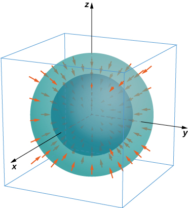
Find the total flux across S with \(p=0.\)
Show that for \(p=3\) the flux across S is independent of a and b.
The net flux is zero.
Glossary
- flux integral
- another name for a surface integral of a vector field; the preferred term in physics and engineering
- grid curves
- curves on a surface that are parallel to grid lines in a coordinate plane
- heat flow
- a vector field proportional to the negative temperature gradient in an object
- mass flux
- the rate of mass flow of a fluid per unit area, measured in mass per unit time per unit area
- orientation of a surface
- if a surface has an “inner” side and an “outer” side, then an orientation is a choice of the inner or the outer side; the surface could also have “upward” and “downward” orientations
- parameter domain (parameter space)
- the region of the uv plane over which the parameters u and v vary for parameterization \(\text{r}(u,v)=\langle x(u,v),y(u,v),z(u,v)\rangle\)
- parameterized surface (parametric surface)
- a surface given by a description of the form \(\text{r}(u,v)=\langle x(u,v),y(u,v),z(u,v)\rangle ,\) where the parameters u and v vary over a parameter domain in the uv-plane
- regular parameterization
- parameterization \(\text{r}(u,v)=\langle x(u,v),y(u,v),z(u,v)\rangle\) such that \({\text{r}}_{u}\,\times \,{\text{r}}_{v}\) is not zero for any point \((u,v)\) in the parameter domain
- surface area
- the area of surface S given by the surface integral \(∫{∫}_{S}dS\)
- surface integral
- an integral of a function over a surface
- surface integral of a scalar-valued function
- a surface integral in which the integrand is a scalar function
- surface integral of a vector field
- a surface integral in which the integrand is a vector field