Section 6.4Green's Theorem
In this section, we examine Green’s theorem, which is an extension of the Fundamental Theorem of Calculus to two dimensions. Green’s theorem has two forms: a circulation form and a flux form, both of which require region D in the double integral to be simply connected. However, we will extend Green’s theorem to regions that are not simply connected.
Put simply, Green’s theorem relates a line integral around a simply closed plane curve C and a double integral over the region enclosed by C. The theorem is useful because it allows us to translate difficult line integrals into more simple double integrals, or difficult double integrals into more simple line integrals.
Extending the Fundamental Theorem of Calculus
Recall that the Fundamental Theorem of Calculus says that
\[{∫}_{a}^{b}{F}^{\prime }(x)dx=F(b)-F(a).\]
As a geometric statement, this equation says that the integral over the region below the graph of \({F}^{\prime }(x)\) and above the line segment \([a,b]\) depends only on the value of F at the endpoints a and b of that segment. Since the numbers a and b are the boundary of the line segment \([a,b],\) the theorem says we can calculate integral \({∫}_{a}^{b}F\prime (x)dx\) based on information about the boundary of line segment \([a,b]\) (Figure 1). The same idea is true of the Fundamental Theorem for Line Integrals:
\[{∫}_{C}\nabla f·d\text{r}=f(\text{r}(b))-f(\text{r}(a)).\]
When we have a potential function (an “antiderivative”), we can calculate the line integral based solely on information about the boundary of curve C.
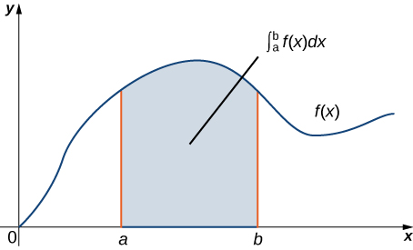
Green’s theorem takes this idea and extends it to calculating double integrals. Green’s theorem says that we can calculate a double integral over region D based solely on information about the boundary of D. Green’s theorem also says we can calculate a line integral over a simple closed curve C based solely on information about the region that C encloses. In particular, Green’s theorem connects a double integral over region D to a line integral around the boundary of D.
Circulation Form of Green’s Theorem
The first form of Green’s theorem that we examine is the circulation form. This form of the theorem relates the vector line integral over a simple, closed plane curve C to a double integral over the region enclosed by C. Therefore, the circulation of a vector field along a simple closed curve can be transformed into a double integral and vice versa.
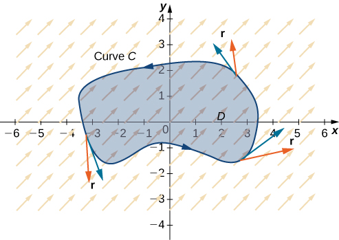
Let D be an open, simply connected region with a boundary curve C that is a piecewise smooth, simple closed curve oriented counterclockwise (Figure 2). Let \(\text{F}=\langle P,Q\rangle\) be a vector field with component functions that have continuous partial derivatives on D. Then,
\[{∫}_{C}\text{F}·d\text{r}={∫}_{C}Pdx+Qdy={∬}_{D}({Q}_{x}-{P}_{y})dA.\]
Notice that Green’s theorem can be used only for a two-dimensional vector field F. If F is a three-dimensional field, then Green’s theorem does not apply. Since
\[{∫}_{C}Pdx+Qdy={∫}_{C}\text{F}·\text{T}ds,\]
this version of Green’s theorem is sometimes referred to as the tangential form of Green’s theorem.
The proof of Green’s theorem is rather technical, and beyond the scope of this text. Here we examine a proof of the theorem in the special case that D is a rectangle. For now, notice that we can quickly confirm that the theorem is true for the special case in which \(\text{F}=\langle P,Q\rangle\) is conservative. In this case,
\[{∫}_{C}Pdx+Qdy=0\]
because the circulation is zero in conservative vector fields. By (see original), F satisfies the cross-partial condition, so \({P}_{y}={Q}_{x}.\) Therefore,
\[{∬}_{D}({Q}_{x}-{P}_{y})dA={∬}_{D}0dA=0={∫}_{C}Pdx+Qdy,\]
which confirms Green’s theorem in the case of conservative vector fields.
Proof
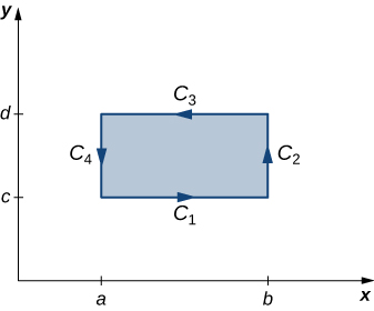
Let’s now prove that the circulation form of Green’s theorem is true when the region D is a rectangle. Let D be the rectangle \([a,b]\,\times \,[c,d]\) oriented counterclockwise. Then, the boundary C of D consists of four piecewise smooth pieces \({C}_{1},\) \({C}_{2},\) \({C}_{3},\) and \({C}_{4}\) (Figure 3). We parameterize each side of D as follows:
\[\begin{array}{lll}{C}_{1}\text{:}\,{\text{r}}_{1}(t) & = & \langle t,c\rangle ,a\le t\le b \\ {C}_{2}\text{:}\,{\text{r}}_{2}(t) & = & \langle b,t\rangle ,c\le t\le d \\ \text{-}{C}_{3}\text{:}\,{\text{r}}_{3}(t) & = & \langle t,d\rangle ,a\le t\le b \\ \text{-}{C}_{4}\text{:}\,{\text{r}}_{4}(t) & = & \langle a,t\rangle ,c\le t\le d.\end{array}\]
Then,
\[\begin{array}{ll}{∫}_{C}\text{F}·d\text{r} & ={∫}_{{C}_{1}}\text{F}·d\text{r}+{∫}_{{C}_{2}}\text{F}·d\text{r}+{∫}_{{C}_{3}}\text{F}·d\text{r}+{∫}_{{C}_{4}}\text{F}·d\text{r} \\ & ={∫}_{{C}_{1}}\text{F}·d\text{r}+{∫}_{{C}_{2}}\text{F}·d\text{r}-{∫}_{\text{-}{C}_{3}}\text{F}·d\text{r}-{∫}_{\text{-}{C}_{4}}\text{F}·d\text{r} \\ & ={∫}_{a}^{b}\text{F}({\text{r}}_{1}(t))·{\text{r}}_{1'}(t)dt+{∫}_{c}^{d}\text{F}({\text{r}}_{2}(t))·{\text{r}}_{2'}(t)dt \\ & \,\text{-}{∫}_{a}^{b}\text{F}({\text{r}}_{3}(t))·{\text{r}}_{3'}(t)dt-{∫}_{c}^{d}\text{F}({\text{r}}_{4}(t))·{\text{r}}_{4'}(t)dt \\ & ={∫}_{a}^{b}P(t,c)dt+{∫}_{c}^{d}Q(b,t)dt-{∫}_{a}^{b}P(t,d)dt-{∫}_{c}^{d}Q(a,t)dt \\ & ={∫}_{a}^{b}(P(t,c)-P(t,d))dt+{∫}_{c}^{d}(Q(b,t)-Q(a,t))dt \\ & =\text{-}{∫}_{a}^{b}(P(t,d)-P(t,c))dt+{∫}_{c}^{d}(Q(b,t)-Q(a,t))dt.\end{array}\]
By the Fundamental Theorem of Calculus,
\[P(t,d)-P(t,c)={∫}_{c}^{d}\frac{∂}{∂y}P(t,y)dy\,\text{and}\,Q(b,t)-Q(a,t)={∫}_{a}^{b}\frac{∂}{∂x}Q(x,t)dx.\]
Therefore,
\[\begin{array}{l} \\ \\ \\ \\ \,\text{-}{∫}_{a}^{b}(P(t,d)-P(t,c))dt+{∫}_{c}^{d}(Q(b,t)-Q(a,t))dt \\ =\text{-}{∫}_{a}^{b}{∫}_{c}^{d}\frac{∂}{∂y}P(t,y)dydt+{∫}_{c}^{d}{∫}_{a}^{b}\frac{∂}{∂x}Q(x,t)dxdt.\end{array}\]
But,
\[\begin{array}{ll}-{∫}_{a}^{b}{∫}_{c}^{d}\frac{∂}{∂y}P(t,y)dydt+{∫}_{c}^{d}{∫}_{a}^{b}\frac{∂}{∂x}Q(x,t)dxdt & =\text{-}{∫}_{a}^{b}{∫}_{c}^{d}\frac{∂}{∂y}P(x,y)dydx+{∫}_{c}^{d}{∫}_{a}^{b}\frac{∂}{∂x}Q(x,y)dxdy \\ & ={∫}_{a}^{b}{∫}_{c}^{d}({Q}_{x}-{P}_{y})dydx \\ & =∫{∫}_{D}({Q}_{x}-{P}_{y})dA.\end{array}\]
Therefore, \({∫}_{C}\text{F}·d\text{r}=∫{∫}_{D}({Q}_{x}-{P}_{y})dA\) and we have proved Green’s theorem in the case of a rectangle.
To prove Green’s theorem over a general region D, we can decompose D into many tiny rectangles and use the proof that the theorem works over rectangles. The details are technical, however, and beyond the scope of this text.
□
Calculate the line integral
\[{∫}_{C}{x}^{2}ydx+(y-3)dy,\]
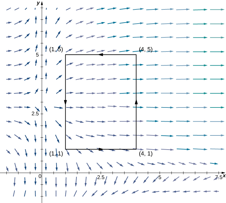
where C is a rectangle with vertices \((1,1),\) \((4,1),\) \((4,5),\) and \((1,5)\) oriented counterclockwise.
Identify \(P\) and \(Q\), compute \(Q_x-P_y\), then set up the double integral of that quantity over the rectangle.
Let \(\text{F}(x,y)=\langle P(x,y),Q(x,y)\rangle =\langle {x}^{2}y,y-3\rangle .\) Then, \({Q}_{x}=0\) and \({P}_{y}={x}^{2}.\) Therefore, \({Q}_{x}-{P}_{y}=\text{-}{x}^{2}.\)
Let D be the rectangular region enclosed by C (Figure 4). By Green’s theorem,
\[\begin{array}{ll}{∫}_{C}{x}^{2}ydx+(y-3)dy & ={∬}_{D}({Q}_{x}-{P}_{y})dA \\ & =∫{∫}_{D}\text{-}{x}^{2}dA={∫}_{1}^{5}{∫}_{1}^{4}\text{-}{x}^{2}dxdy \\ & ={∫}_{1}^{5}-21dy=-84.\end{array}\]
If we were to evaluate this line integral without using Green’s theorem, we would need to parameterize each side of the rectangle, break the line integral into four separate line integrals, and use the methods from Line Integrals to evaluate each integral. Furthermore, since the vector field here is not conservative, we cannot apply the Fundamental Theorem for Line Integrals. Green’s theorem makes the calculation much simpler.
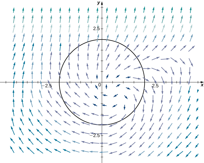
Calculate the work done on a particle by force field
\[\text{F}(x,y)=\langle y+\text{sin}\,x,{e}^{y}-x\rangle \]
as the particle traverses circle \({x}^{2}+{y}^{2}=4\) exactly once in the counterclockwise direction, starting and ending at point \((2,0).\)
Write the work as \({∫}_{C}Pdx+Qdy\), compute \(Q_x-P_y\), and convert the double integral into a multiple of the disk's area.
Let C denote the circle and let D be the disk enclosed by C. The work done on the particle is
\[W={∫}_{C}(y+\text{sin}\,x)dx+({e}^{y}-x)dy.\]
As with Example 1, this integral can be calculated using tools we have learned, but it is easier to use the double integral given by Green’s theorem (Figure 5).
Let \(\text{F}(x,y)=\langle P(x,y),Q(x,y)\rangle =\langle y+\text{sin}\,x,{e}^{y}-x\rangle .\) Then, \({Q}_{x}=-1\) and \({P}_{y}=1.\) Therefore, \({Q}_{x}-{P}_{y}=-2.\)
By Green’s theorem,
\[\begin{array}{ll}W & ={∫}_{C}(y+\text{sin}(x))dx+({e}^{y}-x)dy \\ & ={∬}_{D}({Q}_{x}-{P}_{y})dA={∬}_{D}-2dA \\ & =-2(\text{area}(D))=-2\pi ({2}^{2})=-8\pi .\end{array}\]
Use Green’s theorem to calculate line integral
\[{∫}_{C}\text{sin}({x}^{2})dx+(3x-y)dy,\]
where C is a right triangle with vertices \((-1,2),\) \((4,2),\) and \((4,5)\) oriented counterclockwise.
\(\frac{45}{2}\)
In the preceding two examples, the double integral in Green’s theorem was easier to calculate than the line integral, so we used the theorem to calculate the line integral. In the next example, the double integral is more difficult to calculate than the line integral, so we use Green’s theorem to translate a double integral into a line integral.
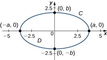
Calculate the area enclosed by ellipse \(\frac{{x}^{2}}{{a}^{2}}+\frac{{y}^{2}}{{b}^{2}}=1\) (Figure 6).
Choose a vector field F with \(Q_x-P_y=1\) (such as \(\langle-y/2,x/2\rangle\)), then use Green's theorem to turn the area integral into a line integral over the ellipse's parameterization.
Let C denote the ellipse and let D be the region enclosed by C. Recall that ellipse C can be parameterized by
\[x=a\,\text{cos}\,t,y=b\,\text{sin}\,t,0\le t\le 2\pi .\]
Calculating the area of D is equivalent to computing double integral \({∬}_{D}dA.\) To calculate this integral without Green’s theorem, we would need to divide D into two regions: the region above the x-axis and the region below. The area of the ellipse is
\[{∫}_{\text{-}a}^{a}{∫}_{0}^{\sqrt{{b}^{2}-{(bx\text{/}a)}^{2}}}dydx+{∫}_{\text{-}a}^{a}{∫}_{\text{-}\sqrt{{b}^{2}-{(bx\text{/}a)}^{2}}}^{0}\,dydx.\]
These two integrals are not straightforward to calculate (although when we know the value of the first integral, we know the value of the second by symmetry). Instead of trying to calculate them, we use Green’s theorem to transform \({∬}_{D}dA\) into a line integral around the boundary C.
Consider vector field
\[\text{F}(x,y)=\langle P,Q\rangle =\langle -\frac{y}{2},\frac{x}{2}\rangle .\]
Then, \({Q}_{x}=\frac{1}{2}\) and \({P}_{y}=-\frac{1}{2},\) and therefore \({Q}_{x}-{P}_{y}=1.\) Notice that F was chosen to have the property that \({Q}_{x}-{P}_{y}=1.\) Since this is the case, Green’s theorem transforms the line integral of F over C into the double integral of 1 over D.
By Green’s theorem,
\[\begin{array}{ll} \\ \\ \\ {∬}_{D}dA & ={∬}_{D}({Q}_{x}-{P}_{y})dA \\ & ={∫}_{C}\text{F}·d\text{r}=\frac{1}{2}{∫}_{C}\text{-}ydx+xdy \\ & =\frac{1}{2}{∫}_{0}^{2\pi }\text{-}b\,\text{sin}\,t(\text{-}a\,\text{sin}\,t)+a(\text{cos}\,t)b\,\text{cos}\,tdt \\ & =\frac{1}{2}{∫}_{0}^{2\pi }ab\,{\text{cos}}^{2}t+ab\,{\text{sin}}^{2}tdt=\frac{1}{2}{∫}_{0}^{2\pi }abdt=\pi ab.\end{array}\]
Therefore, the area of the ellipse is \(\pi ab.\)
In Example 3, we used vector field \(\text{F}(x,y)=\langle P,Q\rangle =\langle -\frac{y}{2},\frac{x}{2}\rangle\) to find the area of any ellipse. The logic of the previous example can be extended to derive a formula for the area of any region D. Let D be any region with a boundary that is a simple closed curve C oriented counterclockwise. If \(\text{F}(x,y)=\langle P,Q\rangle =\langle -\frac{y}{2},\frac{x}{2}\rangle ,\) then \({Q}_{x}-{P}_{y}=1.\) Therefore, by the same logic as in Example 3,
\[\text{area of}\,D={∬}_{D}dA=\frac{1}{2}{∫}_{C}\text{-}ydx+xdy.\]
It’s worth noting that if \(\text{F}=\langle P,Q\rangle\) is any vector field with \({Q}_{x}-{P}_{y}=1,\) then the logic of the previous paragraph works. So. Equation 22 is not the only equation that uses a vector field’s mixed partials to get the area of a region.
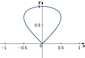
Find the area of the region enclosed by the curve with parameterization \(\text{r}(t)=\langle \text{sin}\,t\,\text{cos}\,t,\text{sin}\,t\rangle ,0\le t\le \pi .\)
\(\frac{2}{3}\)
Flux Form of Green’s Theorem
The circulation form of Green’s theorem relates a double integral over region D to line integral \({∫}_{C}\text{F}·\text{T}ds,\) where C is the boundary of D. The flux form of Green’s theorem relates a double integral over region D to the flux across boundary C. The flux of a fluid across a curve can be difficult to calculate using the flux line integral. This form of Green’s theorem allows us to translate a difficult flux integral into a double integral that is often easier to calculate.
Let D be an open, simply connected region with a boundary curve C that is a piecewise smooth, simple closed curve that is oriented counterclockwise (Figure 7). Let \(\text{F}=\langle P,Q\rangle\) be a vector field with component functions that have continuous partial derivatives on an open region containing D. Then,
\[{∫}_{C}\text{F}·\text{N}ds={∬}_{D}{P}_{x}+{Q}_{y}dA.\]
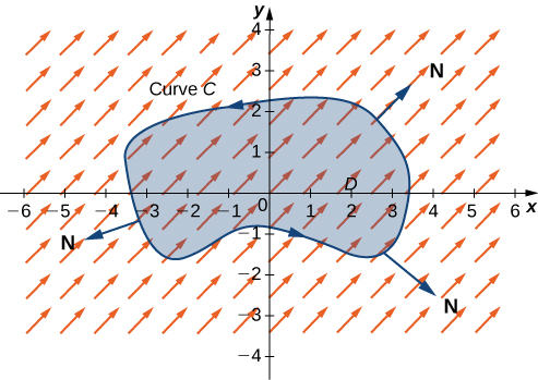
Because this form of Green’s theorem contains unit normal vector N, it is sometimes referred to as the normal form of Green’s theorem.
Proof
Recall that \({∫}_{C}\text{F}·\text{N}ds={∫}_{C}\text{-}Qdx+Pdy.\) Let \(M=\text{-}Q\) and \(N=P.\) By the circulation form of Green’s theorem,
\[\begin{array}{ll}{∫}_{C}\text{-}Qdx+Pdy & ={∫}_{C}Mdx+Ndy \\ & ={∬}_{D}{N}_{x}-{M}_{y}dA \\ & ={∬}_{D}{P}_{x}-{(\text{-}Q)}_{y}dA \\ & ={∬}_{D}{P}_{x}+{Q}_{y}dA.\end{array}\]
□
Let C be a circle of radius r centered at the origin (Figure 8) and let \(\text{F}(x,y)=\langle x,y\rangle .\) Calculate the flux across C.
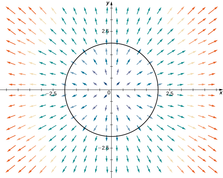
Compute \(P_x+Q_y\) for this field, then use Green's flux form to turn the flux integral into that constant times the disk's area.
Let D be the disk enclosed by C. The flux across C is \({∫}_{C}\text{F}·\text{N}ds.\) We could evaluate this integral using tools we have learned, but Green’s theorem makes the calculation much more simple. Let \(P(x,y)=x\) and \(Q(x,y)=y\) so that \(\text{F}=\langle P,Q\rangle .\) Note that \({P}_{x}=1={Q}_{y},\) and therefore \({P}_{x}+{Q}_{y}=2.\) By Green’s theorem,
\[{∫}_{C}\text{F}·\text{N}ds=∫{∫}_{D}2dA=2∫{∫}_{D}dA.\]
Since \(∫{∫}_{D}dA\) is the area of the circle, \(∫{∫}_{D}dA=\pi {r}^{2}.\) Therefore, the flux across C is \(2\pi {r}^{2}.\)
Let S be the triangle with vertices \((0,0),\) \((1,0),\) and \((0,3)\) oriented clockwise (Figure 9). Calculate the flux of \(\text{F}(x,y)=\langle P(x,y),Q(x,y)\rangle =\langle {x}^{2}+{e}^{y},x+y\rangle\) across S.
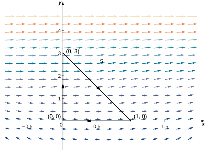
Since S is oriented clockwise, apply Green's theorem to \(-S\) (counterclockwise) and negate the result; compute \(P_x+Q_y\) and set up the iterated integral over the triangle.
To calculate the flux without Green’s theorem, we would need to break the flux integral into three line integrals, one integral for each side of the triangle. Using Green’s theorem to translate the flux line integral into a single double integral is much more simple.
Let D be the region enclosed by S. Note that \({P}_{x}=2x\) and \({Q}_{y}=1;\) therefore, \({P}_{x}+{Q}_{y}=2x+1.\) Green’s theorem applies only to simple closed curves oriented counterclockwise, but we can still apply the theorem because \({∫}_{C}\text{F}·\text{N}ds=\text{-}{∫}_{\text{-}S}\text{F}·\text{N}ds\) and \(\text{-}S\) is oriented counterclockwise. By Green’s theorem, the flux is
\[\begin{array}{ll} \\ \\ \\ {∫}_{C}\text{F}·\text{N}ds & ={∫}_{\text{-}S}\text{F}·\text{N}ds \\ & =\text{-}{∬}_{D}({P}_{x}+{Q}_{y})dA \\ & =\text{-}{∬}_{D}(2x+1)dA.\end{array}\]
Notice that the top edge of the triangle is the line \(y=-3x+3.\) Therefore, in the iterated double integral, the y-values run from \(y=0\) to \(y=-3x+3,\) and we have
\[\begin{array}{ll}\text{-}{∬}_{D}(2x+1)dA & =\text{-}{∫}_{0}^{1}{∫}_{0}^{-3x+3}(2x+1)dydx \\ & =\text{-}{∫}_{0}^{1}(2x+1)(-3x+3)dx=\text{-}{∫}_{0}^{1}(-6{x}^{2}+3x+3)dx \\ & =\text{-}{[-2{x}^{3}+\frac{3{x}^{2}}{2}+3x]}_{0}^{1}=-\frac{5}{2}.\end{array}\]
Calculate the flux of \(\text{F}(x,y)=\langle {x}^{3},{y}^{3}\rangle\) across a unit circle oriented counterclockwise.
\(\frac{3\pi }{2}\)
Water flows from a spring located at the origin. The velocity of the water is modeled by vector field \(\text{v}(x,y)=\langle 5x+y,x+3y\rangle\) m/sec. Find the amount of water per second that flows across the rectangle with vertices \((-1,-2),(1,-2),(1,3),\,\text{and}\,(-1,3),\) oriented counterclockwise (Figure 10).
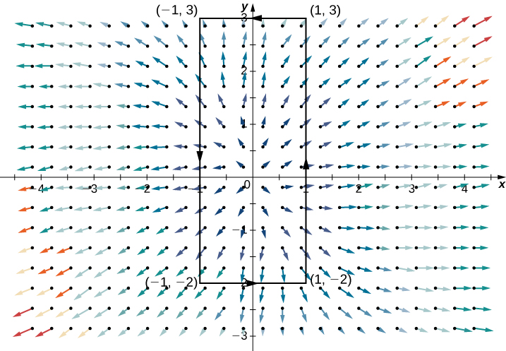
Compute \(P_x+Q_y\) for v and multiply by the area of the rectangle.
Let C represent the given rectangle and let D be the rectangular region enclosed by C. To find the amount of water flowing across C, we calculate flux \({∫}_{C}\text{v}\cdot \text{N}ds.\) Let \(P(x,y)=5x+y\) and \(Q(x,y)=x+3y\) so that \(\text{v}=(P,Q).\) Then, \({P}_{x}=5\) and \({Q}_{y}=3.\) By Green’s theorem,
\[\begin{array}{ll}{∫}_{C}\text{v}\cdot \text{N}ds & ={∬}_{D}({P}_{x}+{Q}_{y})dA \\ & ={∬}_{D}8dA \\ & =8(\text{area of}\,D)=80.\end{array}\]
Therefore, the water flux is 80 m2/sec.
Recall that if vector field F is conservative, then F does no work around closed curves—that is, the circulation of F around a closed curve is zero. In fact, if the domain of F is simply connected, then F is conservative if and only if the circulation of F around any closed curve is zero. If we replace “circulation of F” with “flux of F,” then we get a definition of a source-free vector field. The following statements are all equivalent ways of defining a source-free field \(\text{F}=\langle P,Q\rangle\) on a simply connected domain (note the similarities with properties of conservative vector fields):
- The flux \({∫}_{C}\text{F}·\text{N}ds\) across any closed curve C is zero.
- If \({C}_{1}\) and \({C}_{2}\) are curves in the domain of F with the same starting points and endpoints, then \({∫}_{{C}_{1}}\text{F}·\text{N}ds={∫}_{{C}_{2}}\text{F}·\text{N}ds.\) In other words, flux is independent of path.
- There is a stream function \(g(x,y)\) for F. A stream function for \(\text{F}=\langle P,Q\rangle\) is a function g such that \(P={g}_{y}\) and \(Q=\text{-}{g}_{x}.\) Geometrically, \(\text{F}(a,b)\) is tangential to the level curve of g at \((a,b).\) Since the gradient of g is perpendicular to the level curve of g at \((a,b),\) stream function g has the property \(\text{F}(a,b)·\nabla g(a,b)=0\) for any point \((a,b)\) in the domain of g. (Stream functions play the same role for source-free fields that potential functions play for conservative fields.)
- \({P}_{x}+{Q}_{y}=0\)
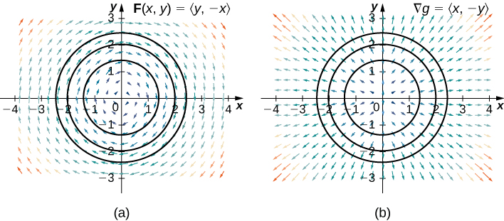
Verify that rotation vector field \(\text{F}(x,y)=\langle y,\text{-}x\rangle\) is source free, and find a stream function for F.
Check \(P_x+Q_y=0\) first, then integrate \(g_y=P\) with respect to y and match \(-g_x\) to Q.
Note that the domain of F is all of \({ℝ}^{2},\) which is simply connected. Therefore, to show that F is source free, we can show any of items 1 through 4 from the previous list to be true. In this example, we show that item 4 is true. Let \(P(x,y)=y\) and \(Q(x,y)=\text{-}x.\) Then \({P}_{x}=0={Q}_{y},\) and therefore \({P}_{x}+{Q}_{y}=0.\) Thus, F is source free.
To find a stream function for F, proceed in the same manner as finding a potential function for a conservative field. Let g be a stream function for F. Then \({g}_{y}=y,\) which implies that
\[g(x,y)=\frac{{y}^{2}}{2}+h(x).\]
Since \(\text{-}{g}_{x}=Q=\text{-}x,\) we have \(h\prime (x)=x.\) Therefore,
\[h(x)=\frac{{x}^{2}}{2}+C.\]
Letting \(C=0\) gives stream function
\[g(x,y)=\frac{{x}^{2}}{2}+\frac{{y}^{2}}{2}.\]
To confirm that g is a stream function for F, note that \({g}_{y}=y=P\) and \(\text{-}{g}_{x}=\text{-}x=Q.\)
Notice that source-free rotation vector field \(\text{F}(x,y)=\langle y,\text{-}x\rangle\) is perpendicular to conservative radial vector field \(\nabla g=\langle x,y\rangle\) (Figure 11).
Find a stream function for vector field \(\text{F}(x,y)=\langle x\,\text{sin}\,y,\text{cos}\,y\rangle .\)
\(g(x,y)=\text{-}x\,\text{cos}\,y\)
Vector fields that are both conservative and source free are important vector fields. One important feature of conservative and source-free vector fields on a simply connected domain is that any potential function \(f\) of such a field satisfies Laplace’s equation \({f}_{xx}+{f}_{yy}=0.\) Laplace’s equation is foundational in the field of partial differential equations because it models such phenomena as gravitational and magnetic potentials in space, and the velocity potential of an ideal fluid. A function that satisfies Laplace’s equation is called a harmonic function. Therefore any potential function of a conservative and source-free vector field is harmonic.
To see that any potential function of a conservative and source-free vector field on a simply connected domain is harmonic, let \(f\) be such a potential function of vector field \(\text{F}=\langle P,Q\rangle .\) Then, \({f}_{x}=P\) and \({f}_{x}=Q\) because \(\nabla f=\text{F}.\) Therefore, \({f}_{xx}={P}_{x}\) and \({f}_{yy}={Q}_{y}.\) Since F is source free, \({f}_{xx}+{f}_{yy}={P}_{x}+{Q}_{y}=0,\) and we have that \(f\) is harmonic.
For vector field \(\text{F}(x,y)=\langle {e}^{x}\text{sin}\,y,{e}^{x}\text{cos}\,y\rangle ,\) verify that the field is both conservative and source free, find a potential function for F, and verify that the potential function is harmonic.
Check the cross-partials for conservativeness and \(P_x+Q_y=0\) for source-free, then build a potential function and confirm \(f_{xx}+f_{yy}=0.\)
Let \(P(x,y)={e}^{x}\text{sin}\,y\) and \(Q(x,y)={e}^{x}\text{cos}\,y.\) Notice that the domain of F is all of two-space, which is simply connected. Therefore, we can check the cross-partials of F to determine whether F is conservative. Note that \({P}_{y}={e}^{x}\text{cos}\,y={Q}_{x},\) so F is conservative. Since \({P}_{x}={e}^{x}\text{sin}\,y\) and \({Q}_{y}=-{e}^{x}\text{sin}\,y,{P}_{x}+{Q}_{y}=0\) and the field is source free.
To find a potential function for F, let \(f\) be a potential function. Then, \(\nabla f=\text{F},\) so \({f}_{x}={e}^{x}\text{sin}\,y.\) Integrating this equation with respect to x gives \(f(x,y)={e}^{x}\text{sin}\,y+h(y).\) Since \({f}_{y}={e}^{x}\text{cos}\,y,\) differentiating \(f\) with respect to y gives \({e}^{x}\text{cos}\,y={e}^{x}\text{cos}\,y+h\prime (y).\) Therefore, we can take \(h(y)=0,\) and \(f(x,y)={e}^{x}\text{sin}\,y\) is a potential function for \(f.\)
To verify that \(f\) is a harmonic function, note that \({f}_{xx}=\frac{∂}{∂x}({e}^{x}\text{sin}\,y)={e}^{x}\text{sin}\,y\) and
\({f}_{yy}=\frac{∂}{∂x}({e}^{x}\text{cos}\,y)=\text{-}{e}^{x}\text{sin}\,y.\) Therefore, \({f}_{xx}+{f}_{yy}=0,\) and \(f\) satisfies Laplace’s equation.
Is the function \(f(x,y)={e}^{x+5y}\) harmonic?
No
Green’s Theorem on General Regions
Green’s theorem, as stated, applies only to regions that are simply connected—that is, Green’s theorem as stated so far cannot handle regions with holes. Here, we extend Green’s theorem so that it does work on regions with finitely many holes (Figure 12).
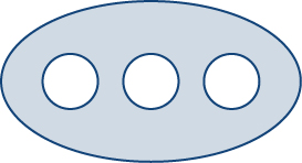
Before discussing extensions of Green’s theorem, we need to go over some terminology regarding the boundary of a region. Let D be a region and let C be a component of the boundary of D. We say that C is positively oriented if, as we walk along C in the direction of orientation, region D is always on our left. Therefore, the counterclockwise orientation of the boundary of a disk is a positive orientation, for example. Curve C is negatively oriented if, as we walk along C in the direction of orientation, region D is always on our right. The clockwise orientation of the boundary of a disk is a negative orientation, for example.
Let D be a region with finitely many holes (so that D has finitely many boundary curves), and denote the boundary of D by \(∂D\) (Figure 13). To extend Green’s theorem so it can handle D, we divide region D into two regions, \({D}_{1}\) and \({D}_{2}\) (with respective boundaries \(∂{D}_{1}\) and \(∂{D}_{2}),\) in such a way that \(D={D}_{1}∪{D}_{2}\) and neither \({D}_{1}\) nor \({D}_{2}\) has any holes (Figure 13).
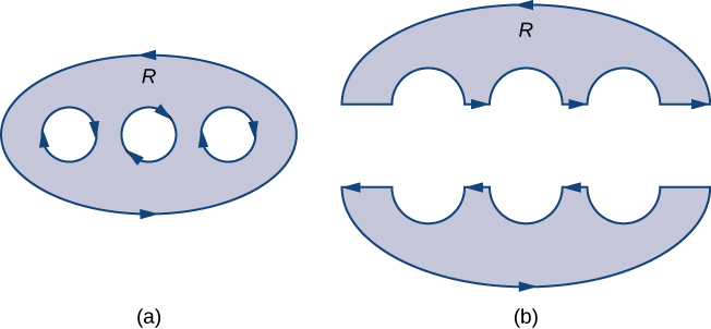
Assume the boundary of D is oriented as in the figure, with the inner holes given a negative orientation and the outer boundary given a positive orientation. The boundary of each simply connected region \({D}_{1}\) and \({D}_{2}\) is positively oriented. If F is a vector field defined on D, then Green’s theorem says that
\[\begin{array}{ll}{∫}_{∂D}\text{F}·d\text{r} & ={∫}_{∂{D}_{1}}\text{F}·d\text{r}+{∫}_{∂{D}_{2}}\text{F}·d\text{r} \\ & ={∬}_{{D}_{1}}{Q}_{x}-{P}_{y}dA+{∬}_{{D}_{2}}{Q}_{x}-{P}_{y}dA \\ & ={∬}_{D}({Q}_{x}-{P}_{y})dA.\end{array}\]
Therefore, Green’s theorem still works on a region with holes.
To see how this works in practice, consider annulus D in Figure 14 and suppose that \(\text{F}=\langle P,Q\rangle\) is a vector field defined on this annulus. Region D has a hole, so it is not simply connected. Orient the outer circle of the annulus counterclockwise and the inner circle clockwise (Figure 14) so that, when we divide the region into \({D}_{1}\) and \({D}_{2},\) we are able to keep the region on our left as we walk along a path that traverses the boundary. Let \({D}_{1}\) be the upper half of the annulus and \({D}_{2}\) be the lower half. Neither of these regions has holes, so we have divided D into two simply connected regions.
We label each piece of these new boundaries as \({P}_{i}\) for some i, as in Figure 14. If we begin at P and travel along the oriented boundary, the first segment is \({P}_{1},\) then \({P}_{2},{P}_{3},\) and \({P}_{4}.\) Now we have traversed \({D}_{1}\) and returned to P. Next, we start at P again and traverse \({D}_{2}.\) Since the first piece of the boundary is the same as \({P}_{4}\) in \({D}_{1},\) but oriented in the opposite direction, the first piece of \({D}_{2}\) is \(\text{-}{P}_{4}.\) Next, we have \({P}_{5},\) then \(\text{-}{P}_{2},\) and finally \({P}_{6}.\)
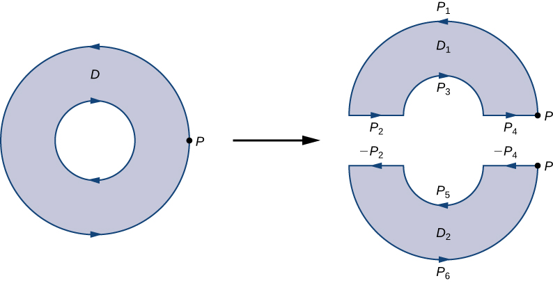
Figure 14 shows a path that traverses the boundary of D. Notice that this path traverses the boundary of region \({D}_{1},\) returns to the starting point, and then traverses the boundary of region \({D}_{2}.\) Furthermore, as we walk along the path, the region is always on our left. Notice that this traversal of the \({P}_{i}\) paths covers the entire boundary of region D. If we had only traversed one portion of the boundary of D, then we cannot apply Green’s theorem to D.
The boundary of the upper half of the annulus, therefore, is \({P}_{1}∪{P}_{2}∪{P}_{3}∪{P}_{4}\) and the boundary of the lower half of the annulus is \(\text{-}{P}_{4}∪{P}_{5}∪-{P}_{2}∪{P}_{6}.\) Then, Green’s theorem implies
\[\begin{array}{ll}{∫}_{∂D}\text{F}·d\text{r} & ={∫}_{{P}_{1}}\text{F}·d\text{r}+{∫}_{{P}_{2}}\text{F}·d\text{r}+{∫}_{{P}_{3}}\text{F}·d\text{r}+{∫}_{{P}_{4}}\text{F}·d\text{r}+{∫}_{\text{-}{P}_{4}}\text{F}·d\text{r}+{∫}_{{P}_{5}}\text{F}·d\text{r}-{∫}_{{P}_{2}}\text{F}·d\text{r}+{∫}_{{P}_{6}}\text{F}·d\text{r} \\ & ={∫}_{{P}_{1}}\text{F}·d\text{r}+{∫}_{{P}_{2}}\text{F}·d\text{r}+{∫}_{{P}_{3}}\text{F}·d\text{r}+{∫}_{{P}_{4}}\text{F}·d\text{r}-{∫}_{{P}_{4}}\text{F}·d\text{r}+{∫}_{{P}_{5}}\text{F}·d\text{r}-{∫}_{{P}_{2}}\text{F}·d\text{r}+{∫}_{{P}_{6}}\text{F}·d\text{r} \\ & ={∫}_{{P}_{1}}\text{F}·d\text{r}+{∫}_{{P}_{3}}\text{F}·d\text{r}+{∫}_{{P}_{5}}\text{F}·d\text{r}+{∫}_{{P}_{6}}\text{F}·d\text{r} \\ & ={∫}_{∂{D}_{1}}\text{F}·d\text{r}+{∫}_{∂{D}_{2}}\text{F}·d\text{r} \\ & ={∬}_{{D}_{1}}({Q}_{x}-{P}_{y})dA+{∬}_{{D}_{2}}({Q}_{x}-{P}_{y})dA \\ & ={∬}_{D}({Q}_{x}-{P}_{y})dA.\end{array}\]
Therefore, we arrive at the equation found in Green’s theorem—namely,
\[{∫}_{∂D}\text{F}·d\text{r}={∬}_{D}({Q}_{x}-{P}_{y})dA.\]
The same logic implies that the flux form of Green’s theorem can also be extended to a region with finitely many holes:
\[{∫}_{C}\text{F}·\text{N}ds={∬}_{D}({P}_{x}+{Q}_{y})dA.\]
Calculate integral
\[{∮}_{∂D}(\text{sin}\,\text{x}-\frac{{y}^{3}}{3})dx+(\frac{{x}^{3}}{3}+\text{sin}\,\text{y})dy,\]
where D is the annulus given by the polar inequalities \(1\le \text{r}\le 2,\) \(0\le θ\le 2\pi .\)
Apply the extended Green's theorem to get \(Q_x-P_y\), then switch to polar coordinates since D is an annulus.
Although D is not simply connected, we can use the extended form of Green’s theorem to calculate the integral. Since the integration occurs over an annulus, we convert to polar coordinates:
\[\begin{array}{ll}{∫}_{∂D}(\text{sin}\,x-\frac{{y}^{3}}{3})dx+(\frac{{x}^{3}}{3}+\text{sin}\,y)dy & ={∬}_{D}({Q}_{x}-{P}_{y})dA \\ & ={∬}_{D}({x}^{2}+{y}^{2})dA \\ & ={∫}_{0}^{2\pi }{∫}_{1}^{2}{r}^{3}drdθ={∫}_{0}^{2\pi }\frac{15}{4}dθ \\ & =\frac{15\pi }{2}.\end{array}\]
Let \(\text{F}=\langle P,Q\rangle =\langle \frac{y}{{x}^{2}+{y}^{2}},-\frac{x}{{x}^{2}+{y}^{2}}\rangle\) and let C be any simple closed curve in a plane oriented counterclockwise. What are the possible values of \({∫}_{C}\text{F}·d\text{r}?\)
Split into two cases based on whether C encloses the origin (where F is undefined), using the extended version of Green's theorem for the second case.
We use the extended form of Green’s theorem to show that \({∫}_{C}\text{F}·d\text{r}\) is either 0 or \(-2\pi\) —that is, no matter how crazy curve C is, the line integral of F along C can have only one of two possible values. We consider two cases: the case when C encompasses the origin and the case when C does not encompass the origin.
Case 1: C Does Not Encompass the Origin
In this case, the region enclosed by C is simply connected because the only hole in the domain of F is at the origin. We showed in our discussion of cross-partials that F satisfies the cross-partial condition. If we restrict the domain of F just to C and the region it encloses, then F with this restricted domain is now defined on a simply connected domain. Since F satisfies the cross-partial property on its restricted domain, the field F is conservative on this simply connected region and hence the circulation \({∫}_{C}\text{F}·d\text{r}\) is zero.
Case 2: C Does Encompass the Origin
In this case, the region enclosed by C is not simply connected because this region contains a hole at the origin. Let \({C}_{1}\) be a circle of radius a centered at the origin so that \({C}_{1}\) is entirely inside the region enclosed by C (Figure 15). Give \({C}_{1}\) a clockwise orientation.
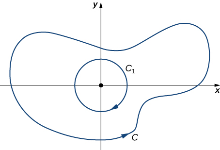
Let D be the region between \({C}_{1}\) and C, and C is orientated counterclockwise. By the extended version of Green’s theorem,
\[\begin{array}{ll}{∫}_{C}\text{F}·d\text{r}+{∫}_{{C}_{1}}\text{F}·d\text{r} & ={∬}_{D}{Q}_{x}-{P}_{y}dA \\ & ={∬}_{D}-\frac{{y}^{2}-{x}^{2}}{{({x}^{2}+{y}^{2})}^{2}}+\frac{{y}^{2}-{x}^{2}}{{({x}^{2}+{y}^{2})}^{2}}dA \\ & =0,\end{array}\]
and therefore
\[{∫}_{C}\text{F}·d\text{r}=-{∫}_{{C}_{1}}\text{F}·d\text{r}.\]
Since \({C}_{1}\) is a specific curve, we can evaluate \({∫}_{{C}_{1}}\text{F}·d\text{r}.\) Let
\[x=a\,\text{cos}\,t,y=-a\,\text{sin}\,t,0\le t\le 2\pi \]
be a parameterization of \({C}_{1}.\) Then,
\[\begin{array}{ll}{∫}_{{C}_{1}}\text{F}·d\text{r} & ={∫}_{0}^{2\pi }\text{F}(\text{r}(t))·\text{r}\prime (t)dt \\ & ={∫}_{0}^{2\pi }\langle -\frac{\text{sin}(t)}{a},-\frac{\text{cos}(t)}{a}\rangle ·\langle \text{-}a\,\text{sin}(t),\text{-}a\,\text{cos}(t)\rangle dt \\ & ={∫}_{0}^{2\pi }{\text{sin}}^{2}(t)+{\text{cos}}^{2}(t)dt={∫}_{0}^{2\pi }dt=2\pi .\end{array}\]
Therefore, \({∫}_{C}\text{F}·d\text{r}=-2\pi .\)
Calculate integral \({∫}_{∂D}\text{F}·d\text{r},\) where D is the annulus given by the polar inequalities \(2\le r\le 5,0\le θ\le 2\pi ,\) and \(\text{F}(x,y)=\langle {x}^{3},5x+{e}^{y}\text{sin}\,y\rangle .\)
\(105\pi\)
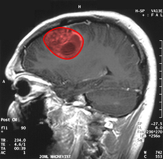
Imagine you are a doctor who has just received a magnetic resonance image of your patient’s brain. The brain has a tumor (Figure 16). How large is the tumor? To be precise, what is the area of the red region? The red cross-section of the tumor has an irregular shape, and therefore it is unlikely that you would be able to find a set of equations or inequalities for the region and then be able to calculate its area by conventional means. You could approximate the area by chopping the region into tiny squares (a Riemann sum approach), but this method always gives an answer with some error.
Instead of trying to measure the area of the region directly, we can use a device called a rolling planimeter to calculate the area of the region exactly, simply by measuring its boundary. In this project you investigate how a planimeter works, and you use Green’s theorem to show the device calculates area correctly.
A rolling planimeter is a device that measures the area of a planar region by tracing out the boundary of that region (Figure 17). To measure the area of a region, we simply run the tracer of the planimeter around the boundary of the region. The planimeter measures the number of turns through which the wheel rotates as we trace the boundary; the area of the shape is proportional to this number of wheel turns. We can derive the precise proportionality equation using Green’s theorem. As the tracer moves around the boundary of the region, the tracer arm rotates and the roller moves back and forth (but does not rotate).
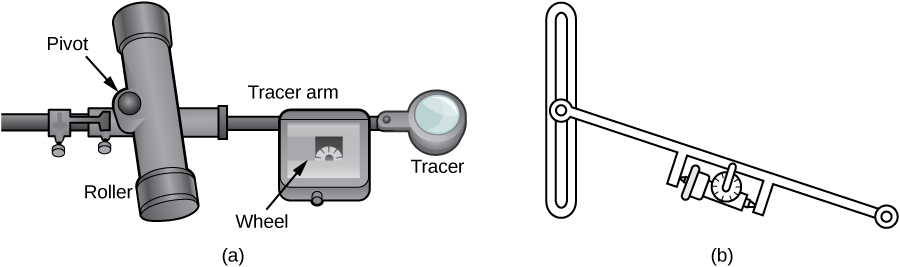
Let C denote the boundary of region D, the area to be calculated. As the tracer traverses curve C, assume the roller moves along the y-axis (since the roller does not rotate, one can assume it moves along a straight line). Use the coordinates \((x,y)\) to represent points on boundary C, and coordinates \((0,Y)\) to represent the position of the pivot. As the planimeter traces C, the pivot moves along the y-axis while the tracer arm rotates on the pivot.
Watch a short animation of a planimeter in action.
Begin the analysis by considering the motion of the tracer as it moves from point \((x,y)\) counterclockwise to point \((x+dx,y+dy)\) that is close to \((x,y)\) (Figure 18). The pivot also moves, from point \((0,Y)\) to nearby point \((0,Y+dY).\) How much does the wheel turn as a result of this motion? To answer this question, break the motion into two parts. First, roll the pivot along the y-axis from \((0,Y)\) to \((0,Y+dY)\) without rotating the tracer arm. The tracer arm then ends up at point \((x,y+dY)\) while maintaining a constant angle \(ϕ\) with the x-axis. Second, rotate the tracer arm by an angle \(dθ\) without moving the roller. Now the tracer is at point \((x+dx,y+dy).\) Let \(l\) be the distance from the pivot to the wheel and let L be the distance from the pivot to the tracer (the length of the tracer arm).
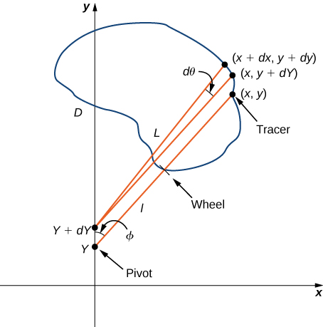
- Explain why the total distance through which the wheel rolls the small motion just described is \(\text{sin}\,ϕdY+ldθ=\frac{x}{L}dY+ldθ.\)
- Show that \({∫}_{C}dθ=0.\)
- Use step 2 to show that the total rolling distance of the wheel as the tracer traverses curve C is
Total wheel roll \(=\frac{1}{L}{∫}_{C}xdY.\)
Now that you have an equation for the total rolling distance of the wheel, connect this equation to Green’s theorem to calculate area D enclosed by C. - Show that \({x}^{2}+{(y-Y)}^{2}={L}^{2}.\)
- Assume the orientation of the planimeter is as shown in Figure 18. Explain why \(Y\le y,\) and use this inequality to show there is a unique value of Y for each point \((x,y)\text{:}\) \(Y=y-\sqrt{{L}^{2}-{x}^{2}}.\)
- Use step 5 to show that \(dY=dy+\frac{x}{\sqrt{{L}^{2}-{x}^{2}}}dx.\)
- Use Green’s theorem to show that \({∫}_{C}\frac{x}{\sqrt{{L}^{2}-{x}^{2}}}dx=0.\)
- Use step 7 to show that the total wheel roll is
Total wheel roll \(=\frac{1}{L}{∫}_{C}xdy.\)
It took a bit of work, but this equation says that the variable of integration Y in step 3 can be replaced with y. - Use Green’s theorem to show that the area of D is \({∫}_{C}xdy.\) The logic is similar to the logic used to show that the area of \(D=\frac{1}{2}{∫}_{C}\text{-}ydx+xdy.\)
- Conclude that the area of D equals the length of the tracer arm multiplied by the total rolling distance of the wheel.
You now know how a planimeter works and you have used Green’s theorem to justify that it works. To calculate the area of a planar region D, use a planimeter to trace the boundary of the region. The area of the region is the length of the tracer arm multiplied by the distance the wheel rolled.
Key Concepts
- Green’s theorem relates the integral over a connected region to an integral over the boundary of the region. Green’s theorem is a version of the Fundamental Theorem of Calculus in one higher dimension. (See Example 1.)
- Green’s Theorem comes in two forms: a circulation form and a flux form. In the circulation form, the integrand is \(\text{F}·\text{T}.\) In the flux form, the integrand is \(\text{F}·\text{N}.\) (See Example 1 and Example 4.)
- Green’s theorem can be used to transform a difficult line integral into an easier double integral, or to transform a difficult double integral into an easier line integral. (See Example 3.)
- A vector field is source free if it has a stream function. The flux of a source-free vector field across a closed curve is zero, just as the circulation of a conservative vector field across a closed curve is zero. (See Example 7.)
Key Equations
| Green’s theorem, circulation form | \({∫}_{C}Pdx+Qdy={∬}_{D}{Q}_{x}-{P}_{y}dA,\) where C is the boundary of D |
| Green’s theorem, flux form | \({∫}_{C}\text{F}·\text{N}ds={∬}_{D}{P}_{x}+{Q}_{y}dA\) |
| Green’s theorem, extended version | \({∫}_{∂D}\text{F}·d\text{r}={∬}_{D}{Q}_{x}-{P}_{y}dA\) |
Section Exercises
For the following exercises, evaluate the line integrals by applying Green’s theorem.
\({∫}_{C}^{}2xydx+(x+y)dy,\) where C is the path from (0, 0) to (1, 1) along the graph of \(y={x}^{3}\) and from (1, 1) to (0, 0) along the graph of \(y=x\) oriented in the counterclockwise direction
\({∫}_{C}^{}2xydx+(x+y)dy,\) where C is the boundary of the region lying between the graphs of \(y=0\) and \(y=4-{x}^{2}\) oriented in the counterclockwise direction
\({∫}_{C}^{}2xydx+(x+y)dy=\frac{32}{3}\)
\({∫}_{C}^{}2\,\text{arctan}(\frac{y}{x})dx+\text{ln}({x}^{2}+{y}^{2})dy,\) where C is defined by \(x=4+2\,\text{cos}\,θ,y=4\,\text{sin}\,θ\) oriented in the counterclockwise direction
\({∫}_{C}^{}\text{sin}\,x\,\text{cos}\,ydx+(xy+\text{cos}\,x\,\text{sin}\,y)dy\text{,}\) where C is the boundary of the region lying between the graphs of \(y=x\) and \(y=\sqrt{x}\) oriented in the counterclockwise direction
\({∫}_{C}^{}\text{sin}\,x\,\text{cos}\,ydx+(xy+\text{cos}\,x\,\text{sin}\,y)dy=\frac{1}{12}\)
\({∫}_{C}^{}xydx+(x+y)dy,\) where C is the boundary of the region lying between the graphs of \({x}^{2}+{y}^{2}=1\) and \({x}^{2}+{y}^{2}=9\) oriented in the counterclockwise direction
\({∫}_{C}(\text{-}ydx+xdy),\) where C consists of line segment C1 from \((-1,0)\) to (1, 0), followed by the semicircular arc C2 from (1, 0) back to (–1, 0)
\({∫}_{C}(\text{-}ydx+xdy)=\pi\)
For the following exercises, use Green’s theorem.
Let C be the curve consisting of line segments from (0, 0) to (1, 1) to (0, 1) and back to (0, 0). Find the value of \({∫}_{C}xydx+\sqrt{{y}^{2}+1}dy.\)
Evaluate line integral \({∫}_{C}x{e}^{-2x}dx+({x}^{4}+2{x}^{2}{y}^{2})dy,\) where C is the boundary of the region between circles \({x}^{2}+{y}^{2}=1\) and \({x}^{2}+{y}^{2}=4,\) and is a positively oriented curve.
\({∫}_{C}x{e}^{-2x}dx+({x}^{4}+2{x}^{2}{y}^{2})dy=0\)
Find the counterclockwise circulation of field \(\text{F}(x,y)=xy\text{i}+{y}^{2}\text{j}\) around and over the boundary of the region enclosed by curves \(y={x}^{2}\) and \(y=x\) in the first quadrant and oriented in the counterclockwise direction.
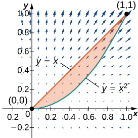
Evaluate \({∫}_{C}{y}^{3}dx-{x}^{3}{y}^{2}dy,\) where C is the positively oriented circle of radius 2 centered at the origin.
\({∫}_{C}{y}^{3}dx-{x}^{3}ydy=-20\pi\)
Evaluate \({∫}_{C}{y}^{3}dx-{x}^{3}dy,\) where C includes the two circles of radius 2 and radius 1 centered at the origin, both with positive orientation.
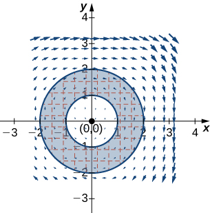
Calculate \({∫}_{C}\text{-}{x}^{2}ydx+x{y}^{2}dy,\) where C is a circle of radius 2 centered at the origin and oriented in the counterclockwise direction.
\({∫}_{C}\text{-}{x}^{2}ydx+x{y}^{2}dy=8\pi\)
Calculate integral \({∫}_{C}2[y+x\,\text{sin}(y)]dx+[{x}^{2}\text{cos}(y)-3{y}^{2}]dy\) along triangle C with vertices (0, 0), (1, 0) and (1, 1), oriented counterclockwise, using Green’s theorem.
Evaluate integral \({∫}_{C}({x}^{2}+{y}^{2})dx+2xydy,\) where C is the curve that follows parabola \(y={x}^{2}\,\text{from}\,(0,0)\text{ to }(2,4),\) then the line from (2, 4) to (2, 0), and finally the line from (2, 0) to (0, 0).
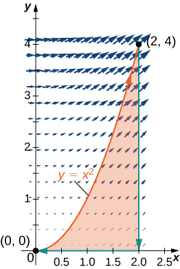
\({∫}_{C}({x}^{2}+{y}^{2})dx+2xydy=0\)
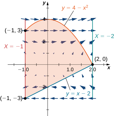
Evaluate line integral \({∫}_{C}(y-\text{sin}(y)\text{cos}(y))dx+2x\,{\text{sin}}^{2}(y)dy,\) where C is oriented in a counterclockwise path around the region bounded by \(x=-1,x=2,y=4-{x}^{2},\) and \(y=x-2.\)
For the following exercises, use Green’s theorem to find the area.
Find the area between ellipse \(\frac{{x}^{2}}{9}+\frac{{y}^{2}}{4}=1\) and circle \({x}^{2}+{y}^{2}=25.\)
\(A=19\pi\)
Find the area of the region enclosed by parametric equation
\[p(θ)=(\text{cos}(θ)-{\text{cos}}^{2}(θ))\text{i}+(\text{sin}(θ)-\text{cos}(θ)\text{sin}(θ))\text{j}\,\text{for}\,0\le θ\le 2\pi .\]
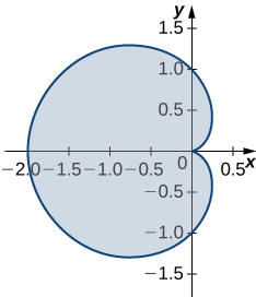
Find the area of the region bounded by hypocycloid \(\text{r}(t)={\text{cos}}^{3}(t)\text{i}+{\text{sin}}^{3}(t)\text{j}.\) The curve is parameterized by \(t\in [0,2\pi ].\)
\(A=\frac{3\pi }{8}\)
Find the area of a pentagon with vertices \((0,4),(4,1),(3,0),(-1,-1),\) and \((-2,2).\)
Use Green’s theorem to evaluate \({∫}_{{C}^{+}}({y}^{2}+{x}^{3})dx+{x}^{4}dy,\) where \({C}^{+}\) is the perimeter of square \([0,1]\,\times \,[0,1]\) oriented counterclockwise.
\({∫}_{C+}({y}^{2}+{x}^{3})dx+{x}^{4}dy=0\)
Use Green’s theorem to prove the area of a disk with radius \(a\) is \(A=\pi {a}^{2}.\)
Use Green’s theorem to find the area of one loop of a four-leaf rose \(r=3\,\text{sin}\,2θ.\) (Hint: \(xdy-ydx={r}^{2}dθ).\)
\(A=\frac{9\pi }{8}\)
Use Green’s theorem to find the area under one arch of the cycloid given by parametric plane \(x=t-\text{sin}\,t,y=1-\text{cos}\,t,t\ge 0.\)
Use Green’s theorem to find the area of the region enclosed by curve
\[\text{r}(t)={t}^{2}\text{i}+(\frac{{t}^{3}}{3}-t)\text{j}\text{,}\,-\sqrt{3}\le t\le \sqrt{3}.\]
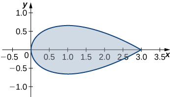
\(A=\frac{8\sqrt{3}}{5}\)
[T] Verify Green’s theorem by using a computer algebra system to evaluate the integral \({∫}_{C}x{e}^{y}dx+{e}^{x}dy,\) where C is the circle given by \({x}^{2}+{y}^{2}=4\) and is oriented in the counterclockwise direction.
Evaluate \({∫}_{C}({x}^{2}y-2xy+{y}^{2})ds,\) where C is the boundary of the unit square \(0\le x\le 1\text{,}\,0\le y\le 1\text{,}\) traversed counterclockwise. Use \(ds = dx + dy\) for this exercise.
\({∫}_{C}({x}^{2}y-2xy+{y}^{2})ds=\frac{1}{2}\)
Evaluate \({∫}_{C}^{}\frac{\text{-}(y+2)dx+(x-1)dy}{{(x-1)}^{2}+{(y+2)}^{2}}\text{,}\) where C is any simple closed curve with an interior that does not contain point \((1,-2)\) traversed counterclockwise.
Evaluate \({∫}_{C}^{}\frac{xdx+ydy}{{x}^{2}+{y}^{2}},\) where C is any piecewise, smooth simple closed curve enclosing the origin, traversed counterclockwise.
\({∫}_{C}^{}\frac{xdx+ydy}{{x}^{2}+{y}^{2}}=0\)
For the following exercises, use Green’s theorem to calculate the work done by force F on a particle that is moving counterclockwise around closed path C.
\(\text{F}(x,y)=xy\text{i}+(x+y)\text{j},\) \(C:{x}^{2}+{y}^{2}=4\)
\(\text{F}(x,y)=({x}^{3\text{/}2}-3y)\text{i}+(6x+5\sqrt{y})\text{j},\) C : boundary of a triangle with vertices (0, 0), (5, 0), and (0, 5)
\(W=\frac{225}{2}\)
Evaluate \({∫}_{C}(2{x}^{3}-{y}^{3})dx+({x}^{3}+{y}^{3})dy,\) where C is a unit circle oriented in the counterclockwise direction.
A particle starts at point \((-2,0),\) moves along the x-axis to (2, 0), and then travels along semicircle \(y=\sqrt{4-{x}^{2}}\) to the starting point. Use Green’s theorem to find the work done on this particle by force field \(\text{F}(x,y)=x\text{i}+({x}^{3}+3x{y}^{2})\text{j}.\)
\(W=12\pi\)
David and Sandra are skating on a frictionless pond in the wind. David skates on the inside, going along a circle of radius 2 in a counterclockwise direction. Sandra skates once around a circle of radius 3, also in the counterclockwise direction. Suppose the force of the wind at point \((x,y)\) \((x,y)\) \((x,y)\) is \(\text{F}(x,y)=({x}^{2}y+10y)\text{i}+({x}^{3}+2x{y}^{2})\text{j}.\) Use Green’s theorem to determine who does more work.
Use Green’s theorem to find the work done by force field \(\text{F}(x,y)=(3y-4x)\text{i}+(4x-y)\text{j}\) when an object moves once counterclockwise around ellipse \(4{x}^{2}+{y}^{2}=4.\)
\(W=2\pi\)
Use Green’s theorem to evaluate line integral \({∫}_{C}{e}^{2x}\text{sin}\,2ydx+{e}^{2x}\text{cos}\,2ydy,\) where C is ellipse \(9{(x-1)}^{2}+4{(y-3)}^{2}=36\) oriented counterclockwise.
Evaluate line integral \({∫}_{C}{y}^{2}dx+{x}^{2}dy,\) where C is the boundary of a triangle with vertices \((0,0),(1,1),\,\text{and}\,(1,0),\) with the counterclockwise orientation.
\({∫}_{C}{y}^{2}dx+{x}^{2}dy=\frac{1}{3}\)
Use Green’s theorem to evaluate line integral \({∫}_{C}\text{h}·d\text{r}\) if \(\text{h}(x,y)={e}^{y}\text{i}-\text{sin}\,\pi x\text{j},\) where C is a triangle with vertices (1, 0), (0, 1), and (–1, 0) traversed counterclockwise.
Use Green’s theorem to evaluate line integral \({∫}_{C}^{}\sqrt{1+{x}^{3}}dx+2xydy\) where C is a triangle with vertices (0, 0), (1, 0), and (1, 3) oriented clockwise.
\({∫}_{C}^{}\sqrt{1+{x}^{3}}dx+2xydy=-3\)
Use Green’s theorem to evaluate line integral \({∫}_{C}^{}{x}^{2}ydx-x{y}^{2}dy\) where C is a circle \({x}^{2}+{y}^{2}=4\) oriented counterclockwise.
Use Green’s theorem to evaluate line integral \({∫}_{C}^{}(3y-{e}^{\text{sin}\,x})dx+(7x+\sqrt{{y}^{4}+1})dy\) where C is circle \({x}^{2}+{y}^{2}=9\) oriented in the counterclockwise direction.
\({∫}_{C}^{}(3y-{e}^{\text{sin}\,x})dx+(7x+\sqrt{{y}^{4}+1})dy=36\pi\)
Use Green’s theorem to evaluate line integral \({∫}_{C}^{}(3x-5y)dx+(x-6y)dy\text{,}\) where C is ellipse \(\frac{{x}^{2}}{4}+{y}^{2}=1\) and is oriented in the counterclockwise direction.
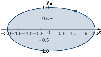
Let C be a triangular closed curve from (0, 0) to (1, 0) to (1, 1) and finally back to (0, 0). Let \(\text{F}(x,y)=4y\text{i}+6{x}^{2}\text{j}.\) Use Green’s theorem to evaluate \({∫}_{C}\text{F}·d\text{r}.\)
\({∫}_{C}\text{F}·d\text{r}=2\)
Use Green’s theorem to evaluate line integral \({∫}_{C}ydx-xdy\text{,}\) where C is circle \({x}^{2}+{y}^{2}={a}^{2}\) oriented in the clockwise direction.
Use Green’s theorem to evaluate line integral \({∫}_{C}(y+x)dx+(x+\text{sin}\,y)dy\text{,}\) where C is any smooth simple closed curve joining the origin to itself oriented in the counterclockwise direction.
\({∫}_{C}(y+x)dx+(x+\text{sin}\,y)dy=0\)
Use Green’s theorem to evaluate line integral \({∫}_{C}(y-\text{ln}({x}^{2}+{y}^{2}))dx+(2\,\text{arctan}\,\frac{y}{x})dy,\) where C is the positively oriented circle \({(x-2)}^{2}+{(y-3)}^{2}=1.\)
Use Green’s theorem to evaluate \({∫}_{C}xydx+{x}^{3}{y}^{3}dy,\) where C is a triangle with vertices (0, 0), (1, 0), and (1, 2) with positive orientation.
\({∫}_{C}xydx+{x}^{3}{y}^{3}dy=\frac{22}{21}\)
Use Green’s theorem to evaluate line integral \({∫}_{C}^{}\text{sin}\,ydx+x\,\text{cos}\,ydy,\) where C is ellipse \({x}^{2}+xy+{y}^{2}=1\) oriented in the counterclockwise direction.
Let \(\text{F}(x,y)=(\text{cos}({x}^{5}))-\frac{1}{3}{y}^{3}\text{i}+\frac{1}{3}{x}^{3}\text{j}.\) Find the counterclockwise circulation \({∫}_{C}\text{F}·d\text{r},\) where C is a curve consisting of the line segment joining \((-2,0)\,\text{and}\,(-1,0)\text{,}\) half circle \(y=\sqrt{1-{x}^{2}},\) the line segment joining (1, 0) and (2, 0), and half circle \(y=\sqrt{4-{x}^{2}}.\)
\({∫}_{C}\text{F}·d\text{r}=\frac{15\pi }{4}\)
Use Green’s theorem to evaluate line integral \({∫}_{C}^{}\text{sin}({x}^{3})dx+2y{e}^{{x}^{2}}dy,\) where C is a triangular closed curve that connects the points (0, 0), (2, 2), and (0, 2) counterclockwise.
Let C be the boundary of square \(0\le x\le \pi \text{,}\,0\le y\le \pi \text{,}\) traversed counterclockwise. Use Green’s theorem to find \({∫}_{C}^{}\text{sin}(x+y)dx+\text{cos}(x+y)dy.\)
\({∫}_{C}^{}\text{sin}(x+y)dx+\text{cos}(x+y)dy=4\)
Use Green’s theorem to evaluate line integral \({∫}_{C}^{}\text{F}·d\text{r},\) where \(\text{F}(x,y)=({y}^{2}-{x}^{2})\text{i}+({x}^{2}+{y}^{2})\text{j},\) and C is a triangle bounded by \(y=0\text{,}\,x=3,\,\text{and}\,y=x\text{,}\) oriented counterclockwise.
Use Green’s Theorem to evaluate integral \({∫}_{C}^{}\text{F}·d\text{r},\) where \(\text{F}(x,y)=(x{y}^{2})\text{i}+x\text{j},\) and C is a unit circle oriented in the counterclockwise direction.
\({∫}_{C}^{}\text{F}·d\text{r}=\pi\)
Use Green’s theorem in a plane to evaluate line integral \({∫}_{C}(xy+{y}^{2})dx+{x}^{2}dy,\) where C is a closed curve of a region bounded by \(y=x\,\text{and}\,y={x}^{2}\) oriented in the counterclockwise direction.
Calculate the outward flux of \(\text{F}=\text{-}x\text{i}+2y\text{j}\) over a square with corners \((\pm 1,\pm 1),\) where the unit normal is outward pointing and oriented in the counterclockwise direction.
\({∫}_{C}\text{F}·\hat{N}ds=4\)
[T] Let C be circle \({x}^{2}+{y}^{2}=4\) oriented in the counterclockwise direction. Evaluate \({∫}_{C}[(3y-{e}^{\text{tan}-{1}_{x}})dx+(7x+\sqrt{{y}^{4}+1})dy]\) using a computer algebra system.
Find the flux of field \(\text{F}=\text{-}x\text{i}+y\text{j}\) across \({x}^{2}+{y}^{2}=16\) oriented in the counterclockwise direction.
\({∫}_{C}\text{F}·\text{N}ds=0\)
Let \(\text{F}=({y}^{2}-{x}^{2})\text{i}+({x}^{2}+{y}^{2})\text{j},\) and let C be a triangle bounded by \(y=0,x=3,\) and \(y=x\) oriented in the counterclockwise direction. Find the outward flux of F through C.
[T] Let C be unit circle \({x}^{2}+{y}^{2}=1\) traversed once counterclockwise. Evaluate \({∫}_{C}[\text{-}{y}^{3}+\text{sin}(xy)+xy\,\text{cos}(xy)]dx+[{x}^{3}+{x}^{2}\text{cos}(xy)]dy\) by using a computer algebra system.
\({∫}_{C}[\text{-}{y}^{3}+\text{sin}(xy)+xy\,\text{cos}(xy)]dx+[{x}^{3}+{x}^{2}\text{cos}(xy)]dy=4.7124\)
[T] Find the outward flux of vector field \(\text{F}=x{y}^{2}\text{i}+{x}^{2}y\text{j}\) across the boundary of annulus \(R=\{(x,y):1\le {x}^{2}+{y}^{2}\le 4\}=\{(r,θ):1\le r\le 2,0\le θ\le 2\pi \}\) using a computer algebra system.
Consider region R bounded by parabolas \(y={x}^{2}\,\text{and}\,x={y}^{2}.\) Let C be the boundary of R oriented counterclockwise. Use Green’s theorem to evaluate \({∫}_{C}(y+{e}^{\sqrt{x}})dx+(2x+\text{cos}({y}^{2}))dy.\)
\({∫}_{C}(y+{e}^{\sqrt{x}})dx+(2x+\text{cos}({y}^{2}))dy=\frac{1}{3}\)
Glossary
- Green’s theorem
- relates the integral over a connected region to an integral over the boundary of the region
- stream function
- if \(\text{F}=\langle P,Q\rangle\) is a source-free vector field, then stream function g is a function such that \(P={g}_{y}\) and \(Q=\text{-}{g}_{x}\)