Section 6.3Conservative Vector Fields
In this section, we continue the study of conservative vector fields. We examine the Fundamental Theorem for Line Integrals, which is a useful generalization of the Fundamental Theorem of Calculus to line integrals of conservative vector fields. We also show how to test whether a given vector field is conservative, and determine how to build a potential function for a vector field known to be conservative.
Curves and Regions
Before continuing our study of conservative vector fields, we need some geometric definitions. The theorems in the subsequent sections all rely on integrating over certain kinds of curves and regions, so we develop the definitions of those curves and regions here.
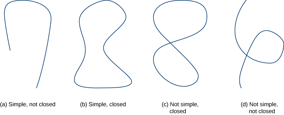
We first define two special kinds of curves: closed curves and simple curves. As we have learned, a closed curve is one that begins and ends at the same point. A simple curve is one that does not cross itself. A curve that is both closed and simple is a simple closed curve (Figure 1).
Curve C is a closed curve if there is a parameterization \(\text{r}(t),a\le t\le b\) of C such that the parameterization traverses the curve exactly once and \(\text{r}(a)=\text{r}(b).\) Curve C is a simple curve if C does not cross itself. That is, C is simple if there exists a parameterization \(\text{r}(t),a\le t\le b\) of C such that r is one-to-one over \((a,b).\) It is possible for \(\text{r}(a)=\text{r}(b),\) meaning that the simple curve is also closed.
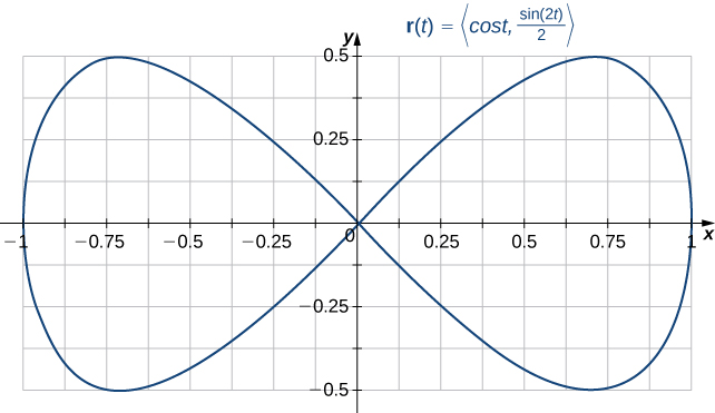
Is the curve with parameterization \(\text{r}(t)=\langle \text{cos}\,t,\frac{\text{sin}(2t)}{2}\rangle ,0\le t\le 2\pi\) a simple closed curve?
Check whether \(\text{r}(0)=\text{r}(2\pi)\) for closedness, then look for two distinct \(t\) values in \([0,2\pi)\) giving the same point.
Note that \(\text{r}(0)=\langle 1,0\rangle =\text{r}(2\pi );\) therefore, the curve is closed. The curve is not simple, however. To see this, note that \(\text{r}(\frac{\pi }{2})=\langle 0,0\rangle =\text{r}(\frac{3\pi }{2}),\) and therefore the curve crosses itself at the origin (Figure 2).
Is the curve given by parameterization \(\text{r}(t)=\langle 2\,\text{cos}\,t,3\,\text{sin}\,t\rangle ,0\le t\le 6\pi ,\) a simple closed curve?
Yes
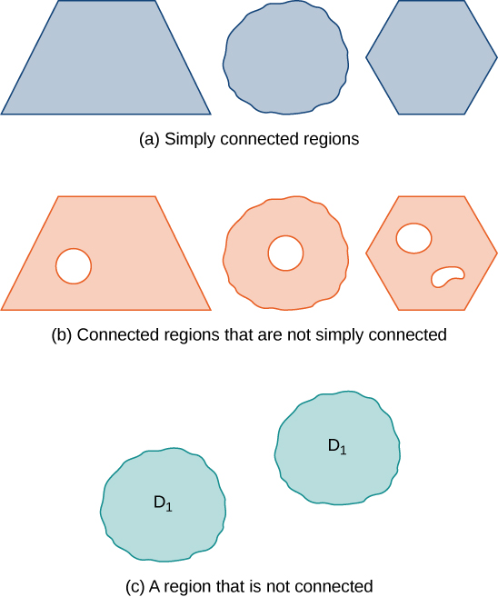
Many of the theorems in this chapter relate an integral over a region to an integral over the boundary of the region, where the region’s boundary is a simple closed curve or a union of simple closed curves. To develop these theorems, we need two geometric definitions for regions: that of a connected region and that of a simply connected region. A connected region is one in which there is a path in the region that connects any two points that lie within that region. A simply connected region is a connected region that does not have any holes in it. These two notions, along with the notion of a simple closed curve, allow us to state several generalizations of the Fundamental Theorem of Calculus later in the chapter. These two definitions are valid for regions in any number of dimensions, but we are only concerned with regions in two or three dimensions.
A region D is a connected region if, for any two points \({P}_{1}\) and \({P}_{2},\) there is a path from \({P}_{1}\) to \({P}_{2}\) with a trace contained entirely inside D. A region D is a simply connected region if D is connected for any simple closed curve C that lies inside D, and curve C can be shrunk continuously to a point while staying entirely inside D. In two dimensions, a region is simply connected if it is connected and has no holes.
All simply connected regions are connected, but not all connected regions are simply connected (Figure 3).
Is the region in the below image connected? Is the region simply connected?
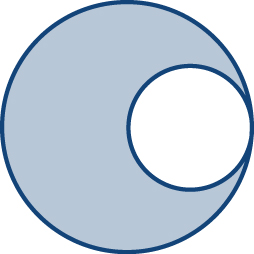
The region in the figure is connected. The region in the figure is not simply connected.
Fundamental Theorem for Line Integrals
Now that we understand some basic curves and regions, let’s generalize the Fundamental Theorem of Calculus to line integrals. Recall that the Fundamental Theorem of Calculus says that if a function \(f\) has an antiderivative F, then the integral of \(f\) from a to b depends only on the values of F at a and at b—that is,
\[{∫}_{a}^{b}f(x)dx=\text{F}(b)-\text{F}(a).\]
If we think of the gradient as a derivative, then the same theorem holds for vector line integrals. We show how this works using a motivational example.
Let \(\text{F}(x,y)=\langle 2x,4y\rangle .\) Calculate \({∫}_{C}\text{F}·d\text{r},\) where C is the line segment from (0,0) to (2,2)(Figure 4).
Parametrize the segment, then compute \(\text{F}(\text{r}(t))·{\text{r}}^{\prime}(t)\) and integrate.
We use (see original) to calculate \({∫}_{C}\text{F}·d\text{r}.\) Curve C can be parameterized by \(\text{r}(t)=\langle 2t,2t\rangle ,0\le t\le 1.\) Then, \(\text{F}(\text{r}(t))=\langle 4t,8t\rangle\) and \({\text{r}}^{\prime }(t)=\langle 2,2\rangle ,\) which implies that
\[\begin{array}{ll}{∫}_{C}\text{F}·d\text{r} & ={∫}_{0}^{1}\langle 4t,8t\rangle ·\langle 2,2\rangle dt \\ & ={∫}_{0}^{1}(8t+16t)dt={∫}_{0}^{1}24t\,dt \\ & ={[12{t}^{2}]}_{0}^{1}=12.\end{array}\]
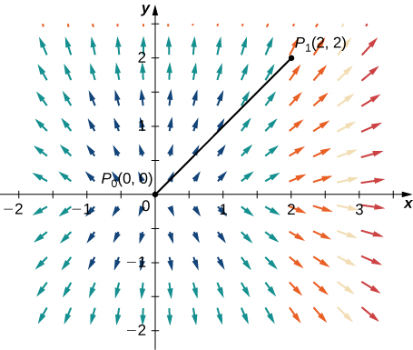
Notice that \(F=\nabla f,\) where \(f(x,y)={x}^{2}+2{y}^{2}.\) If we think of the gradient as a derivative, then \(f\) is an “antiderivative” of F. In the case of single-variable integrals, the integral of derivative \({g}^{\prime }(x)\) is \(g(b)-g(a),\) where a is the start point of the interval of integration and b is the endpoint. If vector line integrals work like single-variable integrals, then we would expect integral F to be \(f({P}_{1})-f({P}_{0}),\) where \({P}_{1}\) is the endpoint of the curve of integration and \({P}_{0}\) is the start point. Notice that this is the case for this example:
\[{∫}_{C}\text{F}·d\text{r}={∫}_{C}\nabla f.d\text{r}=12\]
and
\[f(2,2)-f(0,0)=4+8-0=12.\]
In other words, the integral of a “derivative” can be calculated by evaluating an “antiderivative” at the endpoints of the curve and subtracting, just as for single-variable integrals.
The following theorem says that, under certain conditions, what happened in the previous example holds for any gradient field. The same theorem holds for vector line integrals, which we call the Fundamental Theorem for Line Integrals.
Let C be a piecewise smooth curve with parameterization \(\text{r}(t),a\le t\le b.\) Let \(f\) be a function of two or three variables with first-order partial derivatives that exist and are continuous on C. Then,
\[{∫}_{C}\nabla f.d\text{r}=f(\text{r}(b))-f(\text{r}(a)).\]
Proof
By (see original),
\[{∫}_{C}\nabla f.d\text{r}={∫}_{a}^{b}\nabla f(\text{r}(t)).{\text{r}}^{\prime }(t)dt.\]
By the chain rule,
\[\frac{d}{dt}(f(\text{r}(t))=\nabla f(\text{r}(t)).{\text{r}}^{\prime }(t).\]
Therefore, by the Fundamental Theorem of Calculus,
\[\begin{array}{ll}{∫}_{C}\nabla f.d\text{r} & ={∫}_{a}^{b}\nabla f(\text{r}(t)).{\text{r}}^{\prime }(t)dt \\ & ={∫}_{a}^{b}\frac{d}{dt}(f(\text{r}(t))dt \\ & ={[f(\text{r}(t))]}_{t=a}^{t=b} \\ & =f(\text{r}(b))-f(\text{r}(a)).\end{array}\]
□
We know that if F is a conservative vector field, there are potential functions \(f\) such that \(\nabla f=\text{F}.\) Therefore \({∫}_{C}\text{F}·d\text{r}={∫}_{C}\nabla f·d\text{r}=f(\text{r}(b))-f(\text{r}(a)).\) In other words, just as with the Fundamental Theorem of Calculus, computing the line integral \({∫}_{C}\text{F}·d\text{r},\) where F is conservative, is a two-step process: (1) find a potential function (“antiderivative”) \(f\) for F and (2) compute the value of \(f\) at the endpoints of C and calculate their difference \(f(\text{r}(b))-f(\text{r}(a)).\) Keep in mind, however, there is one major difference between the Fundamental Theorem of Calculus and the Fundamental Theorem for Line Integrals. A function of one variable that is continuous must have an antiderivative. However, a vector field, even if it is continuous, does not need to have a potential function.
Calculate integral \({∫}_{C}\text{F}·d\text{r},\) where \(\text{F}(x,y,z)=\langle 2x\,\text{ln}\,y,\frac{{x}^{2}}{y}+{z}^{2},2yz\rangle\) and C is a curve with parameterization \(\text{r}(t)=\langle {t}^{2},t,t\rangle ,1\le t\le e\)
- without using the Fundamental Theorem of Line Integrals and
- using the Fundamental Theorem of Line Integrals.
For (a), substitute the parameterization directly into \(\text{F}(\text{r}(t))·{\text{r}}^{\prime}(t)\); for (b), use the given potential function and just evaluate it at the endpoints.
- First, let’s calculate the integral without the Fundamental Theorem for Line Integrals and instead use (see original):
Integral \({∫}_{1}^{e}{t}^{3}\text{ln}\,tdt\) requires integration by parts. Let \(u=\text{ln}\,t\) and \(dv={t}^{3}.\) Then \(u=\text{ln}\,t,dv={t}^{3}\)
and
Therefore,
Thus,\[\begin{array}{ll}{∫}_{C}\text{F}·d\text{r} & ={∫}_{1}^{e}\text{F}(\text{r}(t)).{\text{r}}^{'}(t)dt \\ & ={∫}_{1}^{e}⟨2{t}^{2}\text{ln}\,t,\frac{{t}^{4}}{t}+{t}^{2},2{t}^{2}⟩.⟨2t,1,1⟩dt \\ & ={∫}_{1}^{e}(4{t}^{3}\text{ln}\,t+{t}^{3}+3{t}^{2})dt \\ & ={∫}_{1}^{e}4{t}^{3}\text{ln}\,tdt+{∫}_{1}^{e}({t}^{3}+3{t}^{2})dt \\ & ={∫}_{1}^{e}4{t}^{3}\text{ln}\,tdt+{[\frac{{t}^{4}}{4}+{t}^{3}]}_{1}^{e} \\ & =2{∫}_{1}^{e}{t}^{3}\text{ln}\,tdt+\frac{{e}^{4}}{4}+{e}^{3}-\frac{5}{4}.\end{array}\]
\[du=\frac{1}{t}dt,v=\frac{{t}^{4}}{4}.\]
\[\begin{array}{ll}{∫}_{1}^{e}{t}^{3}\text{ln}\,tdt & ={[\frac{{t}^{4}}{4}\text{ln}\,t]}_{1}^{e}-\frac{1}{4}{∫}_{1}^{e}{t}^{3}dt \\ & =\frac{{e}^{4}}{4}-\frac{1}{4}(\frac{{e}^{4}}{4}-\frac{1}{4}).\end{array}\]
\[\begin{array}{ll}{∫}_{C}\text{F}·dr & =4{∫}_{1}^{e}{t}^{3}\text{ln}\,tdt+\frac{{e}^{4}}{4}+{e}^{3}-\frac{5}{4} \\ & =4(\frac{{e}^{4}}{4}-\frac{1}{4}(\frac{{e}^{4}}{4}-\frac{1}{4}))+\frac{{e}^{4}}{4}+{e}^{3}-\frac{5}{4} \\ & ={e}^{4}-\frac{{e}^{4}}{4}+\frac{1}{4}+\frac{{e}^{4}}{4}+{e}^{3}-\frac{5}{4} \\ & ={e}^{4}+{e}^{3}-1.\end{array}\]
- Given that \(f(x,y,z)={x}^{2}\text{ln}\,y+y{z}^{2}\) is a potential function for F, let’s use the Fundamental Theorem for Line Integrals to calculate the integral. Note that
This calculation is much more straightforward than the calculation we did in (a). As long as we have a potential function, calculating a line integral using the Fundamental Theorem for Line Integrals is much easier than calculating without the theorem.\[\begin{array}{ll}{∫}_{C}\text{F}·d\text{r} & ={∫}_{C}\nabla f.d\text{r} \\ & =f(\text{r}(e))-f(\text{r}(1)) \\ & =f({e}^{2},e,e)-f(1,1,1) \\ & ={e}^{4}+{e}^{3}-1.\end{array}\]
Example 3 illustrates a nice feature of the Fundamental Theorem of Line Integrals: it allows us to calculate more easily many vector line integrals. As long as we have a potential function, calculating the line integral is only a matter of evaluating the potential function at the endpoints and subtracting.
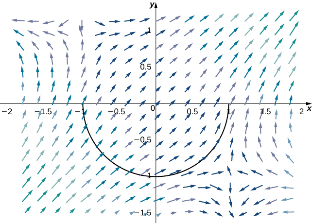
Given that \(f(x,y)={(x-1)}^{2}y+{(y+1)}^{2}x\) is a potential function for \(\text{F}=\langle 2xy-2y+{(y+1)}^{2},{(x-1)}^{2}+2yx+2x\rangle ,\) calculate integral \({∫}_{C}\text{F}·d\text{r},\) where C is the lower half of the unit circle oriented counterclockwise.
2
The Fundamental Theorem for Line Integrals has two important consequences. The first consequence is that if F is conservative and C is a closed curve, then the circulation of F along C is zero—that is, \({∫}_{C}\text{F}·d\text{r}=0.\) To see why this is true, let \(f\) be a potential function for F. Since C is a closed curve, the terminal point r(b) of C is the same as the initial point r(a) of C—that is, \(\text{r}(a)=\text{r}(b).\) Therefore, by the Fundamental Theorem for Line Integrals,
\[\begin{array}{ll}{∫}_{C}\text{F}·d\text{r} & ={∫}_{C}\nabla f·d\text{r} \\ & =f(\text{r}(b))-f(\text{r}(a)) \\ & =f(\text{r}(b))-f(\text{r}(b)) \\ & =0.\end{array}\]
Recall that the reason a conservative vector field F is called “conservative” is because such vector fields model forces in which energy is conserved. We have shown gravity to be an example of such a force. If we think of vector field F in integral \({∫}_{C}\text{F}·d\text{r}\) as a gravitational field, then the equation \({∫}_{C}\text{F}·d\text{r}=0\) follows. If a particle travels along a path that starts and ends at the same place, then the work done by gravity on the particle is zero.
The second important consequence of the Fundamental Theorem for Line Integrals is that line integrals of conservative vector fields are independent of path—meaning, they depend only on the endpoints of the given curve, and do not depend on the path between the endpoints.
Let F be a vector field with domain D. The vector field F is independent of path (or path independent) if \({∫}_{{C}_{1}}\text{F}·d\text{r}={∫}_{{C}_{2}}\text{F}·d\text{r}\) for any paths \({C}_{1}\) and \({C}_{2}\) in D with the same initial and terminal points.
The second consequence is stated formally in the following theorem.
If F is a conservative vector field, then F is independent of path.
Proof
Let D denote the domain of F and let \({C}_{1}\) and \({C}_{2}\) be two paths in D with the same initial and terminal points (Figure 5). Call the initial point \({P}_{1}\) and the terminal point \({P}_{2}.\) Since F is conservative, there is a potential function \(f\) for F. By the Fundamental Theorem for Line Integrals,
\[{∫}_{{C}_{1}}\text{F}·d\text{r}=f({P}_{2})-f({P}_{1})={∫}_{{C}_{2}}\text{F}·d\text{r}.\]
Therefore, \({∫}_{{C}_{1}}\text{F}·d\text{r}={∫}_{{C}_{2}}\text{F}·d\text{r}\) and F is independent of path.
□
![A vector field in two dimensions. The arrows are shorter the closer to the x axis and line x=1.5 they become. The arrows point up, converging around x=1.5 in quadrant 1. That line is approached from the left and from the right. Below, in quadrant 4, the arrows in the rough interval [1,2.5] curve out, away from the given line x=1.5, but do turn back in and converge to x=1.5 above the x axis. Outside of that interval, the arrows go to the left and right horizontally for x values less than 1 and greater than 2.5, respectively. A line is drawn from P_1 at the origin to P_2 at (3,.75) and labeled C_2. C_1 is a simple curve that connects the given endpoints above C_2, C_3 is a simple curve that connects the given endpoints below C_2.](https://raw.githubusercontent.com/openstax/osbooks-calculus-bundle/main/media/CNX_Calc_Figure_16_03_007.jpg)
To visualize what independence of path means, imagine three hikers climbing from base camp to the top of a mountain. Hiker 1 takes a steep route directly from camp to the top. Hiker 2 takes a winding route that is not steep from camp to the top. Hiker 3 starts by taking the steep route but halfway to the top decides it is too difficult for him. Therefore he returns to camp and takes the non-steep path to the top. All three hikers are traveling along paths in a gravitational field. Since gravity is a force in which energy is conserved, the gravitational field is conservative. By independence of path, the total amount of work done by gravity on each of the hikers is the same because they all started in the same place and ended in the same place. The work done by the hikers includes other factors such as friction and muscle movement, so the total amount of energy each one expended is not the same, but the net energy expended against gravity is the same for all three hikers.
We have shown that if F is conservative, then F is independent of path. It turns out that if the domain of F is open and connected, then the converse is also true. That is, if F is independent of path and the domain of F is open and connected, then F is conservative. Therefore, the set of conservative vector fields on open and connected domains is precisely the set of vector fields independent of path.
If F is a continuous vector field that is independent of path and the domain D of F is open and connected, then F is conservative.
Proof
We prove the theorem for vector fields in \({ℝ}^{2}.\) The proof for vector fields in \({ℝ}^{3}\) is similar. To show that \(\text{F}=\langle P,Q\rangle\) is conservative, we must find a potential function \(f\) for F. To that end, let X be a fixed point in D. For any point \((x,y)\) in D, let C be a path from X to \((x,y).\) Define \(f\) \((x,y)\) by \(f(x,y)={∫}_{C}\text{F}·d\text{r}.\) (Note that this definition of \(f\) makes sense only because F is independent of path. If F was not independent of path, then it might be possible to find another path \({C}^{\prime }\) from X to \((x,y)\) such that \({∫}_{C}\text{F}·d\text{r}\ne {∫}_{C}\text{F}·d\text{r},\) and in such a case \(f\) \((x,y)\) would not be a function.) We want to show that \(f\) has the property \(\nabla f=\text{F}.\)
Since domain D is open, it is possible to find a disk centered at \((x,y)\) such that the disk is contained entirely inside D. Let \((a,y)\) with \(a<x\) be a point in that disk. Let C be a path from X to \((x,y)\) that consists of two pieces: \({C}_{1}\) and \({C}_{2}.\) The first piece, \({C}_{1},\) is any path from X to \((a,y)\) that stays inside D; \({C}_{2}\) is the horizontal line segment from \((a,y)\) to \((x,y)\) (Figure 6). Then
\[f(x,y)={∫}_{{C}_{1}}\text{F}·d\text{r}+{∫}_{{C}_{2}}\text{F}·d\text{r}.\]
The first integral does not depend on x, so
\[{f}_{x}=\frac{∂}{∂x}{∫}_{{C}_{2}}\text{F}·d\text{r}.\]
If we parameterize \({C}_{2}\) by \(\text{r}(t)=\langle t,y\rangle ,a\le t\le x,\) then
\[\begin{array}{ll}{f}_{x} & =\frac{∂}{∂x}{∫}_{{C}_{2}}\text{F}·d\text{r} \\ & =\frac{∂}{∂x}{∫}_{a}^{x}\text{F}(\text{r}(t)).{\text{r}}^{'}(t)dt \\ & =\frac{∂}{∂x}{∫}_{a}^{x}\text{F}(\text{r}(t)).\frac{d}{dt}(⟨t,y⟩)dt \\ & =\frac{∂}{∂x}{∫}_{a}^{x}\text{F}(\text{r}(t)).⟨1,0⟩dt \\ & =\frac{∂}{∂x}{∫}_{a}^{x}P(t,y)dt.\end{array}\]
By the Fundamental Theorem of Calculus (part 1),
\[{f}_{x}=\frac{∂}{∂x}{∫}_{a}^{x}P(t,y)dt=P(x,y).\]
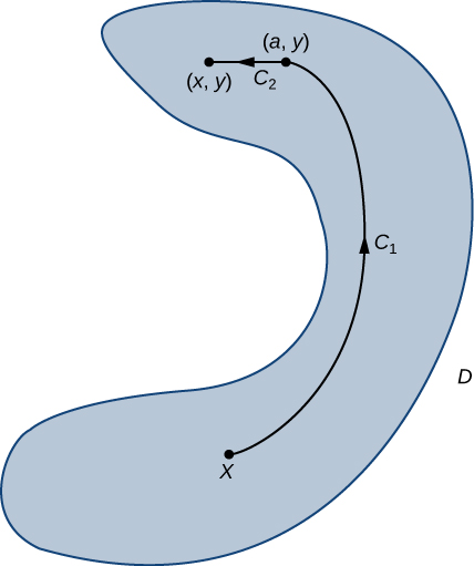
A similar argument using a vertical line segment rather than a horizontal line segment shows that \({f}_{y}=Q(x,y).\)
Therefore \(\nabla f=\text{F}\) and F is conservative.
□
We have spent a lot of time discussing and proving Path Independence of Conservative Fields and The Path Independence Test for Conservative Fields, but we can summarize them simply: a vector field F on an open and connected domain is conservative if and only if it is independent of path. This is important to know because conservative vector fields are extremely important in applications, and these theorems give us a different way of viewing what it means to be conservative using path independence.
Use path independence to show that vector field \(\text{F}(x,y)=\langle {x}^{2}y,y+5\rangle\) is not conservative.
Pick two different paths with the same start and end points, and show the line integral of \(\text{F}\) gives different values along each.
We can indicate that F is not conservative by showing that F is not path independent. We do so by giving two different paths, \({C}_{1}\) and \({C}_{2},\) that both start at \((0,0)\) and end at \((1,1),\) and yet \({∫}_{{C}_{1}}\text{F}·dr\ne {∫}_{{C}_{2}}\text{F}·d\text{r}.\)
Let \({C}_{1}\) be the curve with parameterization \({\text{r}}_{1}(t)=\langle t,t\rangle ,0\le t\le 1\) and let \({C}_{2}\) be the curve with parameterization \({\text{r}}_{2}(t)=\langle t,{t}^{2}\rangle ,0\le t\le 1\) (Figure 7). Then
\[\begin{array}{ll}{∫}_{{C}_{1}}\text{F}·d\text{r} & ={∫}_{0}^{1}\text{F}({\text{r}}_{1}(t))·{\text{r}}_{1}{}^{\prime }(t)dt \\ & ={∫}_{0}^{1}\langle {t}^{3},t+5\rangle ·\langle 1,1\rangle dt={∫}_{0}^{1}({t}^{3}+t+5)dt \\ & ={[\frac{{t}^{4}}{4}+\frac{{t}^{2}}{2}+5t]}_{0}^{1}=\frac{23}{4}\end{array}\]
and
\[\begin{array}{ll}{∫}_{{C}_{2}}\text{F}·d\text{r} & ={∫}_{0}^{1}\text{F}({\text{r}}_{2}(t))·{\text{r}}_{2}\prime (t)dt \\ & ={∫}_{0}^{1}\langle {t}^{4},{t}^{2}+5\rangle ·\langle 1,2t\rangle dt={∫}_{0}^{1}({t}^{4}+2{t}^{3}+10t)dt \\ & ={[\frac{{t}^{5}}{5}+\frac{{t}^{4}}{2}+5{t}^{2}]}_{0}^{1}=\frac{57}{10}.\end{array}\]
Since \({∫}_{{C}_{1}}\text{F}·d\text{r}\ne {∫}_{{C}_{2}}\text{F}·d\text{r},\) the value of a line integral of F depends on the path between two given points. Therefore, F is not independent of path, and F is not conservative.
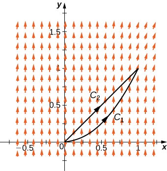
Show that \(\text{F}(x,y)=\langle xy,{x}^{2}{y}^{2}\rangle\) is not path independent by considering the line segment from \((0,0)\) to \((2,2)\) and the piece of the graph of \(y=\frac{{x}^{2}}{2}\) that goes from \((0,0)\) to \((2,2).\)
If \({C}_{1}\) and \({C}_{2}\) represent the two curves, then \({∫}_{{C}_{1}}\text{F}·d\text{r}\ne {∫}_{{C}_{2}}\text{F}·d\text{r}.\)
Conservative Vector Fields and Potential Functions
As we have learned, the Fundamental Theorem for Line Integrals says that if F is conservative, then calculating \({∫}_{C}\text{F}·dr\) has two steps: first, find a potential function \(f\) for F and, second, calculate \(f({P}_{1})-f({P}_{0}),\) where \({P}_{1}\) is the endpoint of C and \({P}_{0}\) is the starting point. To use this theorem for a conservative field F, we must be able to find a potential function \(f\) for F. Therefore, we must answer the following question: Given a conservative vector field F, how do we find a function \(f\) such that \(\nabla f=\text{F}?\) Before giving a general method for finding a potential function, let’s motivate the method with an example.
Find a potential function for \(\text{F}(x,y)=\langle 2x{y}^{3},3{x}^{2}{y}^{2}+\text{cos}(y)\rangle ,\) thereby showing that F is conservative.
Integrate the first component with respect to x, leaving an unknown function of y, then match the y-partial to the second component.
Suppose that \(f(x,y)\) is a potential function for F. Then, \(\nabla f=\text{F},\) and therefore
\[{f}_{x}=2x{y}^{3}\,\text{and}\,{f}_{y}=3{x}^{2}{y}^{2}+\text{cos}\,y.\]
Integrating the equation \({f}_{x}=2x{y}^{3}\) with respect to x yields the equation
\[f(x,y)={x}^{2}{y}^{3}+h(y).\]
Notice that since we are integrating a two-variable function with respect to x, we must add a constant of integration that is a constant with respect to x, but may still be a function of y. The equation \(f(x,y)={x}^{2}{y}^{3}+h(y)\) can be confirmed by taking the partial derivative with respect to x:
\[\frac{∂f}{∂x}=\frac{∂}{∂x}({x}^{2}{y}^{3})+\frac{∂}{∂x}(h(y))=2x{y}^{3}+0=2x{y}^{3}.\]
Since \(f\) is a potential function for F,
\[{f}_{y}=3{x}^{2}{y}^{2}+\text{cos}(y),\]
and therefore
\[3{x}^{2}{y}^{2}+{h}^{\prime }(y)=3{x}^{2}{y}^{2}+\text{cos}(y).\]
This implies that \(h\prime (y)=\text{cos}\,y,\) so \(h(y)=\text{sin}\,y+C.\) Therefore, any function of the form \(f(x,y)={x}^{2}{y}^{3}+\text{sin}(y)+C\) is a potential function. Taking, in particular, \(C=0\) gives the potential function \(f(x,y)={x}^{2}{y}^{3}+\text{sin}(y).\)
To verify that \(f\) is a potential function, note that \(\nabla f=\langle 2x{y}^{3},3{x}^{2}{y}^{2}+\text{cos}\,y\rangle =\text{F}.\)
Find a potential function for \(\text{F}(x,y)=\langle {e}^{x}{y}^{3}+y,3{e}^{x}{y}^{2}+x\rangle .\)
\(f(x,y)={e}^{x}{y}^{3}+xy\)
The logic of the previous example extends to finding the potential function for any conservative vector field in \({ℝ}^{2}.\) Thus, we have the following problem-solving strategy for finding potential functions:
- Integrate P with respect to x. This results in a function of the form \(g(x,y)+h(y),\) where \(h(y)\) is unknown.
- Take the partial derivative of \(g(x,y)+h(y)\) with respect to y, which results in the function \({g}_{y}(x,y)+{h}^{\prime }(y).\)
- Use the equation \({g}_{y}(x,y)+{h}^{\prime }(y)=Q(x,y)\) to find \({h}^{\prime }(y).\)
- Integrate \({h}^{\prime }(y)\) to find \(h(y).\)
- Any function of the form \(f(x,y)=g(x,y)+h(y)+C,\) where C is a constant, is a potential function for F.
We can adapt this strategy to find potential functions for vector fields in \({ℝ}^{3},\) as shown in the next example.
Find a potential function for \(\text{F}(x,y,z)=\langle 2xy,{x}^{2}+2y{z}^{3},3{y}^{2}{z}^{2}+2z\rangle ,\) thereby showing that \(\text{F}\) is conservative.
Integrate the first component with respect to x, then work through y and z in turn, matching each partial derivative.
Suppose that \(f\) is a potential function. Then, \(\nabla f=\text{F}\) and therefore \({f}_{x}=2xy.\) Integrating this equation with respect to x yields the equation \(f(x,y,z)={x}^{2}y+g(y,z)\) for some function g. Notice that, in this case, the constant of integration with respect to x is a function of y and z.
Since \(f\) is a potential function,
\[{x}^{2}+2y{z}^{3}={f}_{y}={x}^{2}+{g}_{y}.\]
Therefore,
\[{g}_{y}=2y{z}^{3}.\]
Integrating this function with respect to y yields
\[g(y,z)={y}^{2}{z}^{3}+h(z)\]
for some function \(h(z)\) of z alone. (Notice that, because we know that g is a function of only y and z, we do not need to write \(g(y,z)={y}^{2}{z}^{3}+h(x,z).)\) Therefore,
\[f(x,y,z)={x}^{2}y+g(y,z)={x}^{2}y+{y}^{2}{z}^{3}+h(z).\]
To find \(f\) , we now must only find h. Since \(f\) is a potential function,
\[3{y}^{2}{z}^{2}+2z={g}_{z}=3{y}^{2}{z}^{2}+{h}^{\prime }(z).\]
This implies that \({h}^{\prime }(z)=2z,\) so \(h(z)={z}^{2}+C.\) Letting \(C=0\) gives the potential function
\[f(x,y,z)={x}^{2}y+{y}^{2}{z}^{3}+{z}^{2}.\]
To verify that \(f\) is a potential function, note that \(\nabla f=\langle 2xy,{x}^{2}+2y{z}^{3},3{y}^{2}{z}^{2}+2z\rangle =\text{F}.\)
Find a potential function for \(\text{F}(x,y,z)=\langle 12{x}^{2},\text{cos}\,y\,\text{cos}\,z,1-\text{sin}\,y\,\text{sin}\,z\rangle .\)
\(f(x,y,z)=4{x}^{3}+\text{sin}\,y\,\text{cos}\,z+z\)
We can apply the process of finding a potential function to a gravitational force. Recall that, if an object has unit mass and is located at the origin, then the gravitational force in \({ℝ}^{2}\) that the object exerts on another object of unit mass at the point \((x,y)\) is given by vector field
\[\text{F}(x,y)=\text{-}G\langle \frac{x}{{({x}^{2}+{y}^{2})}^{3\text{/}2}},\frac{y}{{({x}^{2}+{y}^{2})}^{3\text{/}2}}\rangle ,\]
where G is the universal gravitational constant. In the next example, we build a potential function for F, thus confirming what we already know: that gravity is conservative.
Find a potential function \(f\) for \(\text{F}(x,y)=\text{-}G\langle \frac{x}{{({x}^{2}+{y}^{2})}^{3\text{/}2}},\frac{y}{{({x}^{2}+{y}^{2})}^{3\text{/}2}}\rangle .\)
Integrate \({f}_{x}\) with respect to x using u-substitution with \(u=x^2+y^2\), then find \(h(y)\) from the y-partial.
Suppose that \(f\) is a potential function. Then, \(\nabla f=\text{F}\) and therefore
\[{f}_{x}=\frac{\text{-}Gx}{{({x}^{2}+{y}^{2})}^{3\text{/}2}}.\]
To integrate this function with respect to x, we can use u-substitution. If \(u={x}^{2}+{y}^{2},\) then \(\frac{du}{2}=xdx,\) so
\[\begin{array}{ll}∫\frac{\text{-}Gx}{{({x}^{2}+{y}^{2})}^{3\text{/}2}}dx & =∫\frac{\text{-}G}{2{u}^{3\text{/}2}}du \\ & =\frac{G}{\sqrt{u}}+h(y) \\ & =\frac{G}{\sqrt{{x}^{2}+{y}^{2}}}+h(y)\end{array}\]
for some function \(h(y).\) Therefore,
\[f(x,y)=\frac{G}{\sqrt{{x}^{2}+{y}^{2}}}+h(y).\]
Since \(f\) is a potential function for F,
\[{f}_{y}=\frac{\text{-}Gy}{{({x}^{2}+{y}^{2})}^{3\text{/}2}}.\]
Since \(f(x,y)=\frac{G}{\sqrt{{x}^{2}+{y}^{2}}}+h(y),\) \({f}_{y}\) also equals \(\frac{\text{-}Gy}{{({x}^{2}+{y}^{2})}^{3\text{/}2}}+{h}^{\prime }(y).\)
Therefore,
\[\frac{\text{-}Gy}{{({x}^{2}+{y}^{2})}^{3\text{/}2}}+h\prime (y)=\frac{\text{-}Gy}{{({x}^{2}+{y}^{2})}^{3\text{/}2}},\]
which implies that \({h}^{\prime }(y)=0.\) Thus, we can take \(h(y)\) to be any constant; in particular, we can let \(h(y)=0.\) The function
\[f(x,y)=\frac{G}{\sqrt{{x}^{2}+{y}^{2}}}\]
is a potential function for the gravitational field F. To confirm that \(f\) is a potential function, note that
\[\begin{array}{ll}\nabla f & =\langle -\frac{1}{2}\,\frac{G}{{({x}^{2}+{y}^{2})}^{3\text{/}2}}(2x),-\frac{1}{2}\,\frac{G}{{({x}^{2}+{y}^{2})}^{3\text{/}2}}(2y)\rangle \\ & =\langle \frac{\text{-}Gx}{{({x}^{2}+{y}^{2})}^{3\text{/}2}},\frac{\text{-}Gy}{{({x}^{2}+{y}^{2})}^{3\text{/}2}}\rangle \\ & =\text{F}.\end{array}\]
Find a potential function \(f\) for the three-dimensional gravitational force \(\text{F}(x,y,z)=\langle \frac{\text{-}Gx}{{({x}^{2}+{y}^{2}+{z}^{2})}^{3\text{/}2}},\frac{\text{-}Gy}{{({x}^{2}+{y}^{2}+{z}^{2})}^{3\text{/}2}},\frac{\text{-}Gz}{{({x}^{2}+{y}^{2}+{z}^{2})}^{3\text{/}2}}\rangle .\)
\(f(x,y,z)=\frac{G}{\sqrt{{x}^{2}+{y}^{2}+{z}^{2}}}\)
Testing a Vector Field
Until now, we have worked with vector fields that we know are conservative, but if we are not told that a vector field is conservative, we need to be able to test whether it is conservative. Recall that, if F is conservative, then F has the cross-partial property (see (see original)). That is, if \(\text{F}=\langle P,Q,R\rangle\) is conservative, then \({P}_{y}={Q}_{x},{P}_{z}={R}_{x},\) and \({Q}_{z}={R}_{y}.\) So, if F has the cross-partial property, then is F conservative? If the domain of F is open and simply connected, then the answer is yes.
If \(\text{F}=\langle P,Q,R\rangle\) is a vector field on an open, simply connected region D and \({P}_{y}={Q}_{x},{P}_{z}={R}_{x},\) and \({Q}_{z}={R}_{y}\) throughout D, then F is conservative.
Although a proof of this theorem is beyond the scope of the text, we can discover its power with some examples. Later, we see why it is necessary for the region to be simply connected.
Combining this theorem with the cross-partial property, we can determine whether a given vector field is conservative:
Let \(\text{F}=\langle P,Q,R\rangle\) be a vector field on an open, simply connected region D. Then \({P}_{y}={Q}_{x},{P}_{z}={R}_{x},\) and \({Q}_{z}={R}_{y}\) throughout D if and only if F is conservative.
The version of this theorem in \({ℝ}^{2}\) is also true. If \(\text{F}=\langle P,Q\rangle\) is a vector field on an open, simply connected domain in \({ℝ}^{2},\) then F is conservative if and only if \({P}_{y}={Q}_{x}.\)
Determine whether vector field \(\text{F}(x,y,z)=\langle x{y}^{2}z,{x}^{2}yz,{z}^{2}\rangle\) is conservative.
Since the domain is all of \({ℝ}^{3}\) (simply connected), just check the cross-partials \(Q_z\) and \(R_y\).
Note that the domain of F is all of \({ℝ}^{2}\) and \({ℝ}^{3}\) is simply connected. Therefore, we can use Cross-Partial Property of Conservative Fields to determine whether F is conservative. Let
\[P(x,y,z)=x{y}^{2}z,Q(x,y,z)={x}^{2}yz,\,\text{and}\,R(x,y,z)={z}^{2}.\]
Since \({Q}_{z}={x}^{2}y\) and \({R}_{y}=0,\) the vector field is not conservative.
Determine vector field \(\text{F}(x,y)=\langle x\,\text{ln}(y),\frac{{x}^{2}}{2y}\rangle\) is conservative.
First confirm the domain (\(y>0\)) is simply connected, then check whether \(P_y=Q_x\).
Note that the domain of F is the part of \({ℝ}^{2}\) in which \(y>0.\) Thus, the domain of F is part of a plane above the x-axis, and this domain is simply connected (there are no holes in this region and this region is connected). Therefore, we can use Cross-Partial Property of Conservative Fields to determine whether F is conservative. Let
\[P(x,y)=x\,\text{ln}(y)\,\text{and}\,Q(x,y)=\frac{{x}^{2}}{2y}.\]
Then \({P}_{y}=\frac{x}{y}={Q}_{x}\) and thus F is conservative.
Determine whether \(\text{F}(x,y)=\langle \text{sin}\,x\,\text{cos}\,y,\text{cos}\,x\,\text{sin}\,y\rangle\) is conservative.
It is conservative.
When using Cross-Partial Property of Conservative Fields, it is important to remember that a theorem is a tool, and like any tool, it can be applied only under the right conditions. In the case of Cross-Partial Property of Conservative Fields, the theorem can be applied only if the domain of the vector field is simply connected.
To see what can go wrong when misapplying the theorem, consider the vector field:
\[\text{F}(x,y)=\frac{y}{{x}^{2}+{y}^{2}}\text{i}+\frac{\text{-}x}{{x}^{2}+{y}^{2}}\text{j}.\]
This vector field satisfies the cross-partial property, since
\[\frac{∂}{∂y}(\frac{y}{{x}^{2}+{y}^{2}})=\frac{({x}^{2}+{y}^{2})-y(2y)}{{({x}^{2}+{y}^{2})}^{2}}=\frac{{x}^{2}-{y}^{2}}{{({x}^{2}+{y}^{2})}^{2}}\]
and
\[\frac{∂}{∂x}(\frac{\text{-}x}{{x}^{2}+{y}^{2}})=\frac{\text{-}({x}^{2}+{y}^{2})+x(2x)}{{({x}^{2}+{y}^{2})}^{2}}=\frac{{x}^{2}-{y}^{2}}{{({x}^{2}+{y}^{2})}^{2}}.\]
Since F satisfies the cross-partial property, we might be tempted to conclude that F is conservative. However, F is not conservative. To see this, let
\[\text{r}(t)=\langle \text{cos}\,t,\text{sin}\,t\rangle ,0\le t\le \pi \]
be a parameterization of the upper half of a unit circle oriented counterclockwise (denote this \({C}_{1})\) and let
\[\text{s}(t)=\langle \text{cos}\,t,\text{-}\text{sin}\,t\rangle ,0\le t\le \pi \]
be a parameterization of the lower half of a unit circle oriented clockwise (denote this \({C}_{2}).\) Notice that \({C}_{1}\) and \({C}_{2}\) have the same starting point and endpoint. Since \({\text{sin}}^{2}t+{\text{cos}}^{2}t=1,\)
\[\text{F}(\text{r}(t)).{\text{r}}^{\prime }(t)=\langle \text{sin}(t),\text{-}\text{cos}(t)\rangle .\langle \text{-}\text{sin}(t),\text{cos}(t)\rangle =-1\]
and
\[\begin{array}{ll}\text{F}(s(t))·\text{s}\prime (t) & =\langle \text{-}\text{sin}\,t,\text{-}\text{cos}\,t\rangle ·\langle \text{-}\text{sin}\,t,\text{-}\text{cos}\,t\rangle \\ & ={\text{sin}}^{2}t+{\text{cos}}^{2}t \\ & =1.\end{array}\]
Therefore,
\[{∫}_{{C}_{1}}\text{F}·d\text{r}={∫}_{0}^{\pi }-1dt=\text{-}\pi \,\text{and}\,{∫}_{{C}_{2}}\text{F}·d\text{r}={∫}_{0}^{\pi }1dt=\pi .\]
Thus, \({C}_{1}\) and \({C}_{2}\) have the same starting point and endpoint, but \({∫}_{{C}_{1}}\text{F}·d\text{r}\ne {∫}_{{C}_{2}}\text{F}·d\text{r}.\) Therefore, F is not independent of path and F is not conservative.
To summarize: F satisfies the cross-partial property and yet F is not conservative. What went wrong? Does this contradict Cross-Partial Property of Conservative Fields? The issue is that the domain of F is all of \({ℝ}^{2}\) except for the origin. In other words, the domain of F has a hole at the origin, and therefore the domain is not simply connected. Since the domain is not simply connected, Cross-Partial Property of Conservative Fields does not apply to F.
We close this section by looking at an example of the usefulness of the Fundamental Theorem for Line Integrals. Now that we can test whether a vector field is conservative, we can always decide whether the Fundamental Theorem for Line Integrals can be used to calculate a vector line integral. If we are asked to calculate an integral of the form \({∫}_{C}\text{F}·d\text{r},\) then our first question should be: Is F conservative? If the answer is yes, then we should find a potential function and use the Fundamental Theorem for Line Integrals to calculate the integral. If the answer is no, then the Fundamental Theorem for Line Integrals can’t help us and we have to use other methods, such as using (see original).
Calculate line integral \({∫}_{C}\text{F}·d\text{r},\) where \(\text{F}(x,y,z)=\langle 2x{e}^{y}z+{e}^{x}z,{x}^{2}{e}^{y}z,{x}^{2}{e}^{y}+{e}^{x}\rangle\) and C is any smooth curve that goes from the origin to \((1,1,1).\)
First verify the cross-partials confirm F is conservative, then build a potential function and evaluate it at the two endpoints.
Before trying to compute the integral, we need to determine whether F is conservative and whether the domain of F is simply connected. The domain of F is all of \({ℝ}^{3},\) which is connected and has no holes. Therefore, the domain of F is simply connected. Let
\[P(x,y,z)=2x{e}^{y}z+{e}^{x}z,Q(x,y,z)={x}^{2}{e}^{y}z,\,\text{and}\,R(x,y,z)={x}^{2}{e}^{y}+{e}^{x}\]
so that \(\text{F}=\langle P,Q,R\rangle .\) Since the domain of F is simply connected, we can check the cross partials to determine whether F is conservative. Note that
\[\begin{array}{lll}{P}_{y} & = & 2x{e}^{y}z={Q}_{x} \\ {P}_{z} & = & 2x{e}^{y}+{e}^{x}={R}_{x} \\ {Q}_{z} & = & {x}^{2}{e}^{y}={R}_{y}.\end{array}\]
Therefore, F is conservative.
To evaluate \({∫}_{C}\text{F}·d\text{r}\) using the Fundamental Theorem for Line Integrals, we need to find a potential function \(f\) for F. Let \(f\) be a potential function for F. Then, \(\nabla f=\text{F},\) and therefore \({f}_{x}=2x{e}^{y}z+{e}^{x}z.\) Integrating this equation with respect to x gives \(f(x,y,z)={x}^{2}{e}^{y}z+{e}^{x}z+h(y,z)\) for some function h. Differentiating this equation with respect to y gives \({x}^{2}{e}^{y}z+{h}_{y}=Q={x}^{2}{e}^{y}z,\) which implies that \({h}_{y}=0.\) Therefore, h is a function of z only, and \(f(x,y,z)={x}^{2}{e}^{y}z+{e}^{x}z+h(z).\) To find h, note that \({f}_{z}={x}^{2}{e}^{y}+{e}^{x}+h\prime (z)=R={x}^{2}{e}^{y}+{e}^{x}.\) Therefore, \(h\prime (z)=0\) and we can take \(h(z)=0.\) A potential function for F is \(f(x,y,z)={x}^{2}{e}^{y}z+{e}^{x}z.\)
Now that we have a potential function, we can use the Fundamental Theorem for Line Integrals to evaluate the integral. By the theorem,
\[\begin{array}{ll}{∫}_{C}\text{F}·d\text{r} & ={∫}_{C}\nabla f·d\text{r} \\ & =f(1,1,1)-f(0,0,0) \\ & =2e.\end{array}\]
Notice that if we hadn’t recognized that F is conservative, we would have had to parameterize C and use (see original). Since curve C is unknown, using the Fundamental Theorem for Line Integrals is much simpler.
Calculate integral \({∫}_{C}\text{F}·d\text{r},\) where \(\text{F}(x,y)=\langle \text{sin}\,x\,\text{sin}\,y,5-\text{cos}\,x\,\text{cos}\,y\rangle\) and C is a semicircle with starting point \((0,\pi )\) and endpoint \((0,\text{-}\pi ).\)
\(-10\pi\)
Let \(\text{F}(x,y)=\langle 2x{y}^{2},2{x}^{2}y\rangle\) be a force field. Suppose that a particle begins its motion at the origin and ends its movement at any point in a plane that is not on the x-axis or the y-axis. Furthermore, the particle’s motion can be modeled with a smooth parameterization. Show that F does positive work on the particle.
First find a potential function for F, then apply the Fundamental Theorem for Line Integrals and argue the resulting expression is always positive.
We show that F does positive work on the particle by showing that F is conservative and then by using the Fundamental Theorem for Line Integrals.
To show that F is conservative, suppose \(f(x,y)\) were a potential function for F. Then, \(\nabla f=\text{F}=\langle 2x{y}^{2},2{x}^{2}y\rangle\) and therefore \({f}_{x}=2x{y}^{2}\) and \({f}_{y}=2{x}^{2}y.\) Equation \({f}_{x}=2x{y}^{2}\) implies that \(f(x,y)={x}^{2}{y}^{2}+h(y).\) Deriving both sides with respect to y yields \({f}_{y}=2{x}^{2}y+{h}^{\prime }(y).\) Therefore, \({h}^{\prime }(y)=0\) and we can take \(h(y)=0.\)
If \(f(x,y)={x}^{2}{y}^{2},\) then note that \(\nabla f=\langle 2x{y}^{2},2{x}^{2}y\rangle =\text{F},\) and therefore \(f\) is a potential function for F.
Let \((a,b)\) be the point at which the particle stops is motion, and let C denote the curve that models the particle’s motion. The work done by F on the particle is \({∫}_{C}\text{F}·d\text{r}.\) By the Fundamental Theorem for Line Integrals,
\[\begin{array}{ll}{∫}_{C}\text{F}·d\text{r} & ={∫}_{C}\nabla f·d\text{r} \\ & =f(a,b)-f(0,0) \\ & ={a}^{2}{b}^{2}.\end{array}\]
Since \(a\ne 0\) and \(b\ne 0,\) by assumption, \({a}^{2}{b}^{2}>0.\) Therefore, \({∫}_{C}\text{F}·d\text{r}>0,\) and F does positive work on the particle.
Notice that this problem would be much more difficult without using the Fundamental Theorem for Line Integrals. To apply the tools we have learned, we would need to give a curve parameterization and use (see original). Since the path of motion C can be as exotic as we wish (as long as it is smooth), it can be very difficult to parameterize the motion of the particle.
Let \(\text{F}(x,y)=\langle 4{x}^{3}{y}^{4},4{x}^{4}{y}^{3}\rangle ,\) and suppose that a particle moves from point \((4,4)\) to \((1,1)\) along any smooth curve. Is the work done by F on the particle positive, negative, or zero?
Negative
Key Concepts
- The theorems in this section require curves that are closed, simple, or both, and regions that are connected or simply connected. (See Example 1.)
- The line integral of a conservative vector field can be calculated using the Fundamental Theorem for Line Integrals. This theorem is a generalization of the Fundamental Theorem of Calculus in higher dimensions. Using this theorem usually makes the calculation of the line integral easier. (See Example 3 and Example 10.)
- Conservative fields are independent of path. The line integral of a conservative field depends only on the value of the potential function at the endpoints of the domain curve. (See Example 4.)
- Given vector field F, we can test whether F is conservative by using the cross-partial property. If F has the cross-partial property and the domain is simply connected, then F is conservative (and thus has a potential function). If F is conservative, we can find a potential function by using the Problem-Solving Strategy. (See Example 5 and Example 8.)
- The circulation of a conservative vector field on a simply connected domain over a closed curve is zero.
Key Equations
| Fundamental Theorem for Line Integrals | \({∫}_{C}\nabla f·d\text{r}=f(\text{r}(b))-f(\text{r}(a))\) |
| Circulation of a conservative field over curve C that encloses a simply connected region | \({∫}_{C}\nabla f·d\text{r}=0\) |
Section Exercises
True or False? If vector field F is conservative on the open and connected region D, then line integrals of F are path independent on D, regardless of the shape of D.
True
True or False? Function \(\text{r}(t)=\text{a}+t(\text{b}-\text{a}),\) where \(0\le t\le 1,\) parameterizes the straight-line segment from \(\text{a}\,\text{to}\,\text{b}.\)
True or False? Vector field \(\text{F}(x,y,z)=(y\,\text{sin}\,z)\text{i}+(x\,\text{sin}\,z)\text{j}+(xy\,\text{cos}\,z)\text{k}\) is conservative.
True
True or False? Vector field \(\text{F}(x,y,z)=y\text{i}+(x+z)\text{j}-y\text{k}\) is conservative.
Verify the Fundamental Theorem of Line Integrals for \({∫}_{C}\text{F}·d\text{r}\) by computing the integral using a parameterization and, separately, by finding a potential function for the case when \(\text{F}(x,y)=(2x+2y)\text{i}+(2x+2y)\text{j}\) and C is a portion of circle \({x}^{2}+{y}^{2}=25\) oriented counterclockwise from (5, 0) to (3, 4).
\({∫}_{C}^{}\text{F}·d\text{r}=24\)
[T] Find \({∫}_{C}^{}\text{F}·d\text{r},\) where \(\text{F}(x,y)=(y{e}^{xy}+\text{cos}\,x)\text{i}+(x{e}^{xy}+\frac{1}{{y}^{2}+1})\text{j}\) and C is a portion of curve \(y=\text{sin}\,x\) from \(x=0\) to \(x=\frac{\pi }{2}.\)
[T] Evaluate line integral \({∫}_{C}^{}\text{F}·d\text{r},\) where \(\text{F}(x,y)=({e}^{x}\text{sin}\,y-y)\text{i}+({e}^{x}\text{cos}\,y-x-2)\text{j},\) and C is the path given by \(r(t)=[{t}^{3}\text{sin}\,\frac{\pi t}{2}]\text{i}-[\frac{\pi }{2}\text{cos}(\frac{\pi t}{2}+\frac{\pi }{2})]\text{j}\) for \(0\le t\le 1.\)
\({∫}_{C}^{}\text{F}·d\text{r}=e-\frac{3\pi }{2}\)
For the following exercises, determine whether the vector field is conservative and, if it is, find the potential function.
\(\text{F}(x,y)=2x{y}^{3}\text{i}+3{y}^{2}{x}^{2}\text{j}\)
\(\text{F}(x,y)=(\text{-}y+{e}^{x}\text{sin}\,y)\text{i}+[(x+2){e}^{x}\text{cos}\,y]\text{j}\)
Not conservative
\(\text{F}(x,y)=({e}^{2x}\text{sin}\,y)\text{i}+[{e}^{2x}\text{cos}\,y]\text{j}\)
\(\text{F}(x,y)=(6x+5y)\text{i}+(5x+4y)\text{j}\)
Conservative, \(f(x,y)=3{x}^{2}+5xy+2{y}^{2}\)
\(\text{F}(x,y)=[2x\,\text{cos}(y)-y\,\text{cos}(x)]\text{i}+[\text{-}{x}^{2}\text{sin}(y)-\text{sin}(x)]\text{j}\)
\(\text{F}(x,y)=[y{e}^{x}+\text{sin}(y)]\text{i}+[{e}^{x}+x\,\text{cos}(y)]\text{j}\)
Conservative, \(f(x,y)=y{e}^{x}+x\,\text{sin}(y)\)
For the following exercises, evaluate the line integrals using the Fundamental Theorem of Line Integrals.
\({∫}_{C}(y\text{i}+x\text{j})·d\text{r},\) where C is any path from (0, 0) to (2, 4)
\({∫}_{C}(2ydx+2xdy),\) where C is the line segment from (0, 0) to (4, 4)
\({∫}_{C}(2ydx+2xdy)=32\)
[T] \({∫}_{C}[\text{arctan}\,\frac{y}{x}-\frac{xy}{{x}^{2}+{y}^{2}}]dx+[\frac{{x}^{2}}{{x}^{2}+{y}^{2}}+{e}^{\text{-}y}(1-y)]dy,\) where C is any smooth curve from (1, 1) to \((-1,2)\)
Find the conservative vector field for the potential function
\[f(x,y)=5{x}^{2}+3xy+{10y}^{2}.\]
\(\text{F}(x,y)=(10x+3y)\text{i}+(3x+20y)\text{j}\)
For the following exercises, determine whether the vector field is conservative and, if so, find a potential function.
\(\text{F}(x,y)=(12xy)\text{i}+6({x}^{2}+{y}^{2})\text{j}\)
\(\text{F}(x,y)=({e}^{x}\text{cos}\,y)\text{i}+6({e}^{x}\text{sin}\,y)\text{j}\)
F is not conservative.
\(\text{F}(x,y)=(2xy{e}^{{x}^{2}y})\text{i}+({x}^{2}{e}^{{x}^{2}y})\text{j}\)
\(\text{F}(x,y\text{,}\,z)=(y{e}^{z})\text{i}+(x{e}^{z})\text{j}+(xy{e}^{z})\text{k}\)
F is conservative and a potential function is \(f(x,y\text{,}\,z)=xy{e}^{z}.\)
\(\text{F}(x,y\text{,}\,z)=(\text{sin}\,y)\text{i}-(x\,\text{cos}\,y)\text{j}+\text{k}\)
\(\text{F}(x,y\text{,}\,z)=(-\frac{1}{y})\text{i}+(\frac{x}{{y}^{2}})\text{j}+(2z-1)\text{k}\)
F is conservative and a potential function is \(f(x,y,z)={z}^{2}-z-\frac{x}{y}.\)
\(\text{F}(x,y,z)=3{z}^{2}\text{i}-\text{cos}\,y\text{j}+2xz\text{k}\)
\(\text{F}(x,y\text{,}\,z)=(2xy)\text{i}+({x}^{2}+2yz)\text{j}+{y}^{2}\text{k}\)
F is conservative and a potential function is \(f(x,y\text{,}\,z)={x}^{2}y+{y}^{2}z.\)
\(\text{F}(x,y)=(4{e}^{x}\text{cos}\,y)\text{i}-(4{e}^{x}\text{sin}\,y)\text{j}\)
\(\text{F}(x,y)=(y{e}^{{x}^{2}})\text{i}+({x}^{2}{e}^{{y}^{2}})\text{j}\)
F is conservative and a potential function is \(f(x,y)={e}^{{x}^{2}y}\)
For the following exercises, evaluate the integral using the Fundamental Theorem of Line Integrals.
Evaluate \({∫}_{C}\nabla f·d\text{r},\) where \(f(x,y\text{,}\,z)=\text{cos}(\pi x)+\text{sin}(\pi y)-xyz\) and C is any path that starts at \((1,\frac{1}{2},2)\) and ends at \((2,1,-1).\)
[T] Evaluate \({∫}_{C}\nabla f·d\text{r},\) where \(f(x,y)=xy+{e}^{x}\) and C is a straight line from \((0,0)\) to \((2,1).\)
\({∫}_{C}\text{F}·dr={e}^{2}+1\)
[T] Evaluate \({∫}_{C}\nabla f·d\text{r},\) where \(f(x,y)={x}^{2}y-x\) and C is any path in a plane from (1, 2) to (3, 2).
Evaluate \({∫}_{C}\nabla f·d\text{r},\) where \(f(x,y\text{,}\,z)=xy{z}^{2}-yz\) and C has initial point (1, 2, 3) and terminal point (3, 5, 1).
\({∫}_{C}\text{F}·dr=-2\)
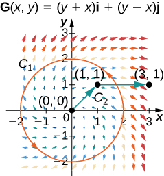
For the following exercises, let \(\text{F}(x,y)=2x{y}^{2}\text{i}+(2y{x}^{2}+2y)\text{j}\) and \(G(x,y)=(y+x)\text{i}+(y-x)\text{j},\) and let C1 be the curve consisting of the circle of radius 2, centered at the origin and oriented counterclockwise, and C2 be the curve consisting of a line segment from (0, 0) to (1, 1) followed by a line segment from (1, 1) to (3, 1).
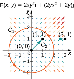
Calculate the line integral of F over C1.
Calculate the line integral of G over C1.
\({∫}_{{C}_{1}}\text{G}·d\text{r}=-8\pi\)
Calculate the line integral of F over C2.
Calculate the line integral of G over C2.
\({∫}_{{C}_{2}}\text{G}·d\text{r}=7\)
[T] Let \(\text{F}(x,y,z)={x}^{2}\text{i}+z\,\text{sin}(yz)\text{j}+y\,\text{sin}(yz)\text{k}.\) Calculate \({∫}_{C}\text{F}·dr,\) where C is a path from \(A=(0,0,1)\) to \(B=(3,1,2).\)
[T] Find line integral \({∫}_{C}\text{F}·dr\) of vector field \(\text{F}(x,y,z)=3{x}^{2}z\text{i}+{z}^{2}\text{j}+({x}^{3}+2yz)\text{k}\) along curve C parameterized by \(r(t)=(\frac{\text{ln}\,t}{\text{ln}\,2})\text{i}+{t}^{3\text{/}2}\text{j}+t\,\text{cos}(\pi t)k\text{,}\,1\le t\le 4.\)
\({∫}_{C}\text{F}·d\text{r}=159\)
For the following exercises, show that the following vector fields are conservative by using a computer. Calculate \({∫}_{C}\text{F}·d\text{r}\) for the given curve.
\(\text{F}=(x{y}^{2}+3{x}^{2}y)\text{i}+(x+y){x}^{2}\text{j};\) C is the curve consisting of line segments from \((1,1)\) to \((0,2)\) to \((3,0).\)
\(\text{F}=\frac{2x}{{y}^{2}+1}\text{i}-\frac{2y({x}^{2}+1)}{{({y}^{2}+1)}^{2}}\text{j};\) C is parameterized by \(x={t}^{3}-1,y={t}^{6}-t,0\le t\le 1.\)
\({∫}_{C}\text{F}·d\text{r}=-1\)
[T] \(\text{F}=[\text{cos}(x{y}^{2})-x{y}^{2}\text{sin}(x{y}^{2})]\text{i}-2{x}^{2}y\,\text{sin}(x{y}^{2})\text{j};\) C is curve \(r(t)=\left({e}^{t},{e}^{t+1}\right),-1\le t\le 0.\)
The mass of Earth is approximately \(6\,\times \,{10}^{27}\text{g}\) and that of the Sun is 330,000 times as much. The gravitational constant is \(6.7\,\times \,{10}^{-8}{\text{cm}}^{3}\text{/}({\text{s}}^{2}·\text{g}).\) The distance of Earth from the Sun is about \(1.5\,\times \,{10}^{12}\text{cm}.\) Compute, approximately, the work necessary to increase the distance of Earth from the Sun by \(1\,\text{cm}.\)
\(4\,\times \,{10}^{29}\text{erg}\)
[T] Let \(\text{F}=({e}^{x}\text{sin}\,y)\text{i}+({e}^{x}\text{cos}\,y)\text{j}+{z}^{2}\text{k}.\) Evaluate the integral \({∫}_{C}\text{F}·dr,\) where \(C\) is the curve \(r(t)=\left(\sqrt{t},{t}^{3},{e}^{\sqrt{t}}\right),0\le t\le 1.\)
[T] Let \(\text{r}:[1,2]\to {ℝ}^{2}\) be given by \(x={e}^{t-1},y=\text{sin}(\frac{\pi }{t}).\) Use a computer to compute the integral \({∫}_{C}\text{F}·d\text{r}={∫}_{C}2x\,\text{cos}\,ydx-{x}^{2}\text{sin}\,ydy,\) where \(\text{F}=(2x\,\text{cos}\,y)\text{i}-({x}^{2}\text{sin}\,y)\text{j}.\)
\({∫}_{C}\text{F}·d\text{r}\approx 2.9923\)
[T] Use a computer algebra system to find the mass of a wire that lies along curve \(\text{r}(t)=({t}^{2}-1)\text{j}+2t\text{k},0\le t\le 1,\) if the density is \(\frac{3}{2}t.\)
Find the circulation and flux of field \(\text{F}=\text{-}y\text{i}+x\text{j}\) around and across the closed semicircular path that consists of semicircular arch \({\text{r}}_{1}(t)=(a\,\text{cos}\,t)\text{i}+(a\,\text{sin}\,t)\text{j},0\le t\le \pi ,\) followed by line segment \({\text{r}}_{2}(t)=t\text{i},\text{-}a\le t\le a.\)
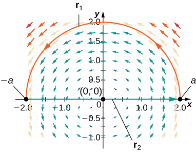
\(\text{circulation}=\pi {a}^{2}\,\text{and flux}=0\)
Compute \({∫}_{C}\text{cos}\,x\,\text{cos}\,ydx-\text{sin}\,x\,\text{sin}\,ydy,\) where \(\text{c}(t)=\left(t,{t}^{2}\right),0\le t\le 1.\)
Complete the proof of The Path Independence Test for Conservative Fields by showing that \({f}_{y}=Q(x,y).\)
Glossary
- closed curve
- a curve that begins and ends at the same point
- connected region
- a region in which any two points can be connected by a path with a trace contained entirely inside the region
- Fundamental Theorem for Line Integrals
- the value of line integral \({∫}_{C}\nabla f·d\text{r}\) depends only on the value of \(f\) at the endpoints of C: \({∫}_{C}\nabla f·d\text{r}=f(\text{r}(b))-f(\text{r}(a))\)
- independence of path
- a vector field F has path independence if \({∫}_{{C}_{1}}\text{F}·d\text{r}={∫}_{{C}_{2}}\text{F}·d\text{r}\) for any curves \({C}_{1}\) and \({C}_{2}\) in the domain of F with the same initial points and terminal points
- simple curve
- a curve that does not cross itself
- simply connected region
- a region that is connected and has the property that any closed curve that lies entirely inside the region encompasses points that are entirely inside the region