Section 6.1Vector Fields
Vector fields are an important tool for describing many physical concepts, such as gravitation and electromagnetism, which affect the behavior of objects over a large region of a plane or of space. They are also useful for dealing with large-scale behavior such as atmospheric storms or deep-sea ocean currents. In this section, we examine the basic definitions and graphs of vector fields so we can study them in more detail in the rest of this chapter.
Examples of Vector Fields
How can we model the gravitational force exerted by multiple astronomical objects? How can we model the velocity of water particles on the surface of a river? Figure 1 gives visual representations of such phenomena.
Figure 1(a) shows a gravitational field exerted by two astronomical objects, such as a star and a planet or a planet and a moon. At any point in the figure, the vector associated with a point gives the net gravitational force exerted by the two objects on an object of unit mass. The vectors of largest magnitude in the figure are the vectors closest to the larger object. The larger object has greater mass, so it exerts a gravitational force of greater magnitude than the smaller object.
Figure 1(b) shows the velocity of a river at points on its surface. The vector associated with a given point on the river’s surface gives the velocity of the water at that point. Since the vectors to the left of the figure are small in magnitude, the water is flowing slowly on that part of the surface. As the water moves from left to right, it encounters some rapids around a rock. The speed of the water increases, and a whirlpool occurs in part of the rapids.
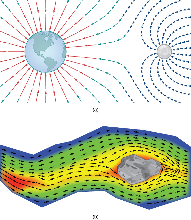
Each figure illustrates an example of a vector field. Intuitively, a vector field is a map of vectors. In this section, we study vector fields in \({ℝ}^{2}\) and \({ℝ}^{3}.\)
A vector field \(\text{F}\) in \({ℝ}^{2}\) is an assignment of a two-dimensional vector \(\text{F}(x,y)\) to each point \((x,y)\) of a subset D of \({ℝ}^{2}.\) The subset D is the domain of the vector field.
A vector field F in \({ℝ}^{3}\) is an assignment of a three-dimensional vector \(\text{F}(x,y,z)\) to each point \((x,y,z)\) of a subset D of \({ℝ}^{3}.\) The subset D is the domain of the vector field.
Vector Fields in \({ℝ}^{2}\)
A vector field in \({ℝ}^{2}\) can be represented in either of two equivalent ways. The first way is to use a vector with components that are two-variable functions:
\[\text{F}(x,y)=\langle P(x,y),Q(x,y)\rangle .\]
The second way is to use the standard unit vectors:
\[\text{F}(x,y)=P(x,y)\text{i}+Q(x,y)\text{j}.\]
A vector field is said to be continuous if its component functions are continuous.
Let \(\text{F}(x,y)=(2{y}^{2}+x-4)\text{i}+\text{cos}(x)\text{j}\) be a vector field in \({ℝ}^{2}.\) Note that this is an example of a continuous vector field since both component functions are continuous. What vector is associated with point \((0,-1)?\)
Substitute \(x=0\) and \(y=-1\) into each component function.
Substitute the point values for x and y:
\[\begin{array}{ll}\text{F}(0,-1) & =(2{(-1)}^{2}+0-4)\text{i}+\text{cos}(0)\text{j} \\ & =-2\text{i}+\text{j}.\end{array}\]
Let \(\text{G}(x,y)={x}^{2}y\text{i}-(x+y)\text{j}\) be a vector field in \({ℝ}^{2}.\) What vector is associated with the point \((-2,3)?\)
\(12\text{i}-\text{j}\)
Drawing a Vector Field
We can now represent a vector field in terms of its components of functions or unit vectors, but representing it visually by sketching it is more complex because the domain of a vector field is in \({ℝ}^{2},\) as is the range. Therefore the “graph” of a vector field in \({ℝ}^{2}\) lives in four-dimensional space. Since we cannot represent four-dimensional space visually, we instead draw vector fields in \({ℝ}^{2}\) in a plane itself. To do this, draw the vector associated with a given point at the point in a plane. For example, suppose the vector associated with point \((4,-1)\) is \(\langle 3,1\rangle .\) Then, we would draw vector \(\langle 3,1\rangle\) at point \((4,-1).\)
We should plot enough vectors to see the general shape, but not so many that the sketch becomes a jumbled mess. If we were to plot the image vector at each point in the region, it would fill the region completely and is useless. Instead, we can choose points at the intersections of grid lines and plot a sample of several vectors from each quadrant of a rectangular coordinate system in \({ℝ}^{2}.\)
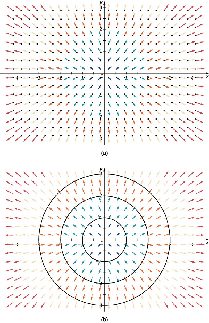
There are two types of vector fields in \({ℝ}^{2}\) on which this chapter focuses: radial fields and rotational fields. Radial fields model certain gravitational fields and energy source fields, and rotational fields model the movement of a fluid in a vortex. In a radial field, all vectors either point directly toward or directly away from the origin. Furthermore, the magnitude of any vector depends only on its distance from the origin. In a radial field, the vector located at point \((x,y)\) is perpendicular to the circle centered at the origin that contains point \((x,y),\) and all other vectors on this circle have the same magnitude.
Sketch the vector field \(\text{F}(x,y)=\frac{x}{2}\,\text{i}+\frac{y}{2}\,\text{j}.\)
Choose a sample of points from each quadrant and compute \(\text{F}\) at each one to build a table before plotting.
To sketch this vector field, choose a sample of points from each quadrant and compute the corresponding vector. The following table gives a representative sample of points in a plane and the corresponding vectors.
| \((x,y)\) | \(\text{F}(x,y)\) | \((x,y)\) | \(\text{F}(x,y)\) | \((x,y)\) | \(\text{F}(x,y)\) |
| \((1,0)\) | \(\langle \frac{1}{2},0\rangle\) | \((2,0)\) | \(\langle 1,0\rangle\) | \((1,1)\) | \(\langle \frac{1}{2},\frac{1}{2}\rangle\) |
| \((0,1)\) | \(\langle 0,\frac{1}{2}\rangle\) | \((0,2)\) | \(\langle 0,1\rangle\) | \((-1,1)\) | \(\langle -\frac{1}{2},\frac{1}{2}\rangle\) |
| \((-1,0)\) | \(\langle -\frac{1}{2},0\rangle\) | \((-2,0)\) | \(\langle -1,0\rangle\) | \((-1,-1)\) | \(\langle -\frac{1}{2},-\frac{1}{2}\rangle\) |
| \((0,-1)\) | \(\langle 0,-\frac{1}{2}\rangle\) | \((0,-2)\) | \(\langle 0,-1\rangle\) | \((1,-1)\) | \(\langle \frac{1}{2},-\frac{1}{2}\rangle\) |
Figure 2(a) shows the vector field. To see that each vector is perpendicular to the corresponding circle, Figure 2(b) shows circles overlain on the vector field.
Draw the radial field \(\text{F}(x,y)=-\frac{x}{3}\,\text{i}-\frac{y}{3}\,\text{j}.\)
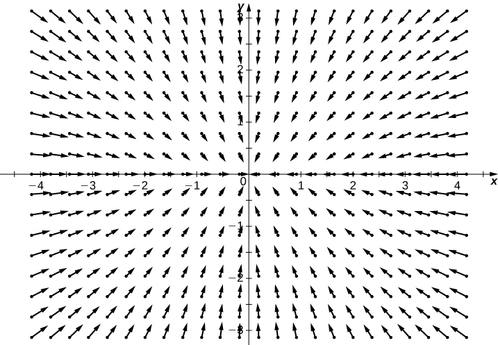
In contrast to radial fields, in a rotational field, the vector at point \((x,y)\) is tangent (not perpendicular) to a circle with radius \(r=\sqrt{{x}^{2}+{y}^{2}}.\) In a standard rotational field, all vectors point either in a clockwise direction or in a counterclockwise direction, and the magnitude of a vector depends only on its distance from the origin. Both of the following examples are clockwise rotational fields, and we see from their visual representations that the vectors appear to rotate around the origin.
Sketch the vector field \(\text{F}(x,y)=\langle y,\text{-}x\rangle .\)
Build a table of sample points \((x,y)\) and their corresponding vectors \(\langle y,-x\rangle\) before plotting.
Create a table (see the one that follows) using a representative sample of points in a plane and their corresponding vectors. Figure 5 shows the resulting vector field.
| \((x,y)\) | \(\text{F}(x,y)\) | \((x,y)\) | \(\text{F}(x,y)\) | \((x,y)\) | \(\text{F}(x,y)\) |
| \((1,0)\) | \(\langle 0,-1\rangle\) | \((2,0)\) | \(\langle 0,-2\rangle\) | \((1,1)\) | \(\langle 1,-1\rangle\) |
| \((0,1)\) | \(\langle 1,0\rangle\) | \((0,2)\) | \(\langle 2,0\rangle\) | \((-1,1)\) | \(\langle 1,1\rangle\) |
| \((-1,0)\) | \(\langle 0,1\rangle\) | \((-2,0)\) | \(\langle 0,2\rangle\) | \((-1,-1)\) | \(\langle -1,1\rangle\) |
| \((0,-1)\) | \(\langle -1,0\rangle\) | \((0,-2)\) | \(\langle -2,0\rangle\) | \((1,-1)\) | \(\langle -1,-1\rangle\) |
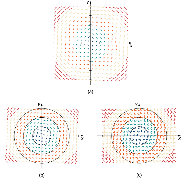
Note that vector \(\text{F}(a,b)=\langle b,\text{-}a\rangle\) points clockwise and is perpendicular to radial vector \(\langle a,b\rangle .\) (We can verify this assertion by computing the dot product of the two vectors: \(\langle a,b\rangle ·\langle \text{-}b,a\rangle =\text{-}ab+ab=0.)\) Furthermore, vector \(\langle b,\text{-}a\rangle\) has length \(r=\sqrt{{a}^{2}+{b}^{2}}.\) Thus, we have a complete description of this rotational vector field: the vector associated with point \((a,b)\) is the vector with length r tangent to the circle with radius r, and it points in the clockwise direction.
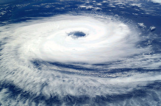
Sketches such as that in Figure 5 are often used to analyze major storm systems, including hurricanes and cyclones. In the northern hemisphere, storms rotate counterclockwise; in the southern hemisphere, storms rotate clockwise. (This is an effect caused by Earth’s rotation about its axis and is called the Coriolis Effect.)
Sketch vector field \(\text{F}(x,y)=\frac{y}{{x}^{2}+{y}^{2}}\,\text{i}-\frac{x}{{x}^{2}+{y}^{2}}\,\text{j}.\)
Check the dot product \(\text{F}(a,b)\cdot(a\text{i}+b\text{j})\) to see each vector is tangent to its circle, then examine \(||\text{F}(a,b)||\) as \((a,b)\to(0,0).\)
To visualize this vector field, first note that the dot product \(\text{F}(a,b)·(a\text{i}+b\text{j})\) is zero for any point \((a,b).\) Therefore, each vector is tangent to the circle on which it is located. Also, as \((a,b)\to (0,0),\) the magnitude of \(\text{F}(a,b)\) goes to infinity. To see this, note that
\[||\text{F}(a,b)||=\sqrt{\frac{{a}^{2}+{b}^{2}}{{({a}^{2}+{b}^{2})}^{2}}}=\sqrt{\frac{1}{{a}^{2}+{b}^{2}}}.\]
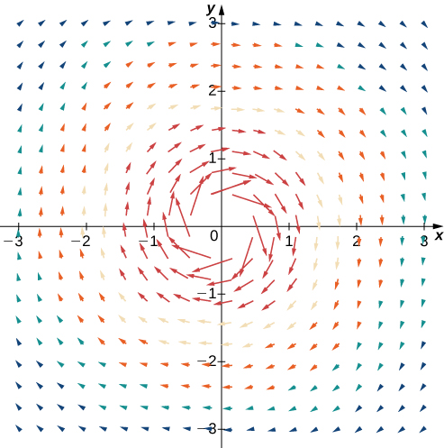
Since \(\frac{1}{{a}^{2}+{b}^{2}}\to \infty\) as \((a,b)\to (0,0),\) then \(||\text{F}(a,b)||\to \infty\) as \((a,b)\to (0,0).\) This vector field looks similar to the vector field in Example 3, but in this case the magnitudes of the vectors close to the origin are large. The table below shows a sample of points and the corresponding vectors, and Figure 5 shows the vector field. Note that this vector field models the whirlpool motion of the river in Figure 1(b). The domain of this vector field is all of \({ℝ}^{2}\) except for point \((0,0).\)
| \((x,y)\) | \(\text{F}(x,y)\) | \((x,y)\) | \(\text{F}(x,y)\) | \((x,y)\) | \(\text{F}(x,y)\) |
| \((1,0)\) | \(\langle 0,-1\rangle\) | \((2,0)\) | \(\langle 0,-\frac{1}{2}\rangle\) | \((1,1)\) | \(\langle \frac{1}{2},-\frac{1}{2}\rangle\) |
| \((0,1)\) | \(\langle 1,0\rangle\) | \((0,2)\) | \(\langle \frac{1}{2},0\rangle\) | \((-1,1)\) | \(\langle \frac{1}{2},\frac{1}{2}\rangle\) |
| \((-1,0)\) | \(\langle 0,1\rangle\) | \((-2,0)\) | \(\langle 0,\frac{1}{2}\rangle\) | \((-1,-1)\) | \(\langle -\frac{1}{2},\frac{1}{2}\rangle\) |
| \((0,-1)\) | \(\langle -1,0\rangle\) | \((0,-2)\) | \(\langle -\frac{1}{2},0\rangle\) | \((1,-1)\) | \(\langle -\frac{1}{2},-\frac{1}{2}\rangle\) |
Sketch vector field \(\text{F}(x,y)=\langle -2y,2x\rangle .\) Is the vector field radial, rotational, or neither?
Rotational
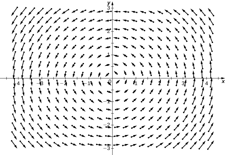
Suppose that \(\text{v}(x,y)=-\frac{2y}{{x}^{2}+{y}^{2}}\,\text{i}+\frac{2x}{{x}^{2}+{y}^{2}}\,\text{j}\) is the velocity field of a fluid. How fast is the fluid moving at point \((1,-1)?\) (Assume the units of speed are meters per second.)
Substitute the point into \(\text{v}\) to get the velocity vector, then take its magnitude.
To find the velocity of the fluid at point \((1,-1),\) substitute the point into v:
\[\text{v}(1,-1)=-\frac{2(-1)}{1+1}\,\text{i}+\frac{2(1)}{1+1}\,\text{j}=\text{i}+\text{j}.\]
The speed of the fluid at \((1,-1)\) is the magnitude of this vector. Therefore, the speed is \(||\text{i}+\text{j}||=\sqrt{2}\) m/sec.
Vector field \(v(x,y)=\langle 4|x|,1\rangle\) models the velocity of water on the surface of a river. What is the speed of the water at point \((2,3)?\) Use meters per second as the units.
\(\sqrt{65}\) m/sec
We have examined vector fields that contain vectors of various magnitudes, but just as we have unit vectors, we can also have a unit vector field. A vector field F is a unit vector field if the magnitude of each vector in the field is 1. In a unit vector field, the only relevant information is the direction of each vector.
Show that the vector field \(\text{G}(x,y)=\langle \frac{y}{\sqrt{{x}^{2}+{y}^{2}}},-\frac{x}{\sqrt{{x}^{2}+{y}^{2}}}\rangle\) is a unit vector field.
Compute the magnitude of \(\text{G}(x,y)\) and show it simplifies to 1.
To show that G is a unit field, we must show that the magnitude of each vector is 1. Note that
\[\begin{array}{ll}\sqrt{{(\frac{y}{\sqrt{{x}^{2}+{y}^{2}}})}^{2}+{(-\frac{x}{\sqrt{{x}^{2}+{y}^{2}}})}^{2}} & =\sqrt{\frac{{y}^{2}}{{x}^{2}+{y}^{2}}+\frac{{x}^{2}}{{x}^{2}+{y}^{2}}} \\ & =\sqrt{\frac{{x}^{2}+{y}^{2}}{{x}^{2}+{y}^{2}}} \\ & =1.\end{array}\]
Therefore, G is a unit vector field.
Is vector field \(\text{F}(x,y)=\langle \text{-}y,x\rangle\) a unit vector field?
No.
Why are unit vector fields important? Suppose we are studying the flow of a fluid, and we care only about the direction in which the fluid is flowing at a given point. In this case, the speed of the fluid (which is the magnitude of the corresponding velocity vector) is irrelevant, because all we care about is the direction of each vector. Therefore, the unit vector field associated with velocity is the field we would study.
If \(\text{F}=\langle P,Q,R\rangle\) is a vector field, then the corresponding unit vector field is \(\langle \frac{P}{||\text{F}||},\frac{Q}{||\text{F}||},\frac{R}{||\text{F}||}\rangle .\) Notice that if \(\text{F}(x,y)=\langle y,\text{-}x\rangle\) is the vector field from Example 3, then the magnitude of F is \(\sqrt{{x}^{2}+{y}^{2}},\) and therefore the corresponding unit vector field is the field G from the previous example.
If F is a vector field, then the process of dividing F by its magnitude to form unit vector field \(\text{F}\text{/}||\text{F}||\) is called normalizing the field F.
Vector Fields in \({ℝ}^{3}\)
We have seen several examples of vector fields in \({ℝ}^{2};\) let’s now turn our attention to vector fields in \({ℝ}^{3}.\) These vector fields can be used to model gravitational or electromagnetic fields, and they can also be used to model fluid flow or heat flow in three dimensions. A two-dimensional vector field can really only model the movement of water on a two-dimensional slice of a river (such as the river’s surface). Since a river flows through three spatial dimensions, to model the flow of the entire depth of the river, we need a vector field in three dimensions.
The extra dimension of a three-dimensional field can make vector fields in \({ℝ}^{3}\) more difficult to visualize, but the idea is the same. To visualize a vector field in \({ℝ}^{3},\) plot enough vectors to show the overall shape. We can use a similar method to visualizing a vector field in \({ℝ}^{2}\) by choosing points in each octant.
Just as with vector fields in \({ℝ}^{2},\) we can represent vector fields in \({ℝ}^{3}\) with component functions. We simply need an extra component function for the extra dimension. We write either
\[\text{F}(x,y,z)=\langle P(x,y,z),Q(x,y,z),R(x,y,z)\rangle \]
or
\[\text{F}(x,y,z)=P(x,y,z)\text{i}+Q(x,y,z)\text{j}+R(x,y,z)\text{k}.\]
Describe vector field \(\text{F}(x,y,z)=\langle 1,1,z\rangle .\)
Start with the xy-plane where \(z=0\), then consider how the vector's z component changes as you move away from it.
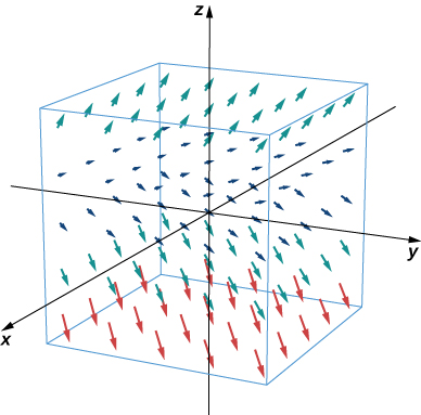
For this vector field, the x and y components are constant, so every point in \({ℝ}^{3}\) has an associated vector with x and y components equal to one. To visualize F, we first consider what the field looks like in the xy-plane. In the xy-plane, \(z=0.\) Hence, each point of the form \((a,b,0)\) has vector \(\langle 1,1,0\rangle\) associated with it. For points not in the xy-plane but slightly above it, the associated vector has a small but positive z component, and therefore the associated vector points slightly upward. For points that are far above the xy-plane, the z component is large, so the vector is almost vertical. Figure 6 shows this vector field.
Sketch vector field \(\text{G}(x,y,z)=\langle 2,\frac{z}{2},1\rangle .\)
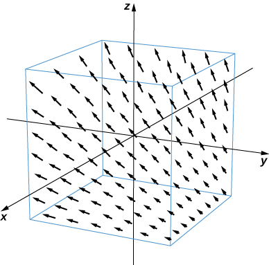
In the next example, we explore one of the classic cases of a three-dimensional vector field: a gravitational field.
Newton’s law of gravitation states that \(\text{F}=\text{-}G\,\frac{{m}_{1}{m}_{2}}{{r}^{2}}\hat{r},\) where G is the universal gravitational constant. It describes the gravitational field exerted by an object (object 1) of mass \({m}_{1}\) located at the origin on another object (object 2) of mass \({m}_{2}\) located at point \((x,y,z).\) Field F denotes the gravitational force that object 1 exerts on object 2, r is the distance between the two objects, and \(\hat{r}\) indicates the unit vector from the first object to the second. The minus sign shows that the gravitational force attracts toward the origin; that is, the force of object 1 is attractive. Sketch the vector field associated with this equation.
Write the distance \(r\) and the unit vector \(\hat{r}\) in terms of \(x,y,z\), then substitute into Newton's law.
Since object 1 is located at the origin, the distance between the objects is given by \(r=\sqrt{{x}^{2}+{y}^{2}+{z}^{2}}.\) The unit vector from object 1 to object 2 is \(\hat{r}=\frac{\langle x,y,z\rangle }{||\langle x,y,z\rangle ||},\) and hence \(\hat{r}=\langle \frac{x}{r},\frac{y}{r},\frac{z}{r}\rangle .\) Therefore, gravitational vector field F exerted by object 1 on object 2 is
\[\text{F}=\text{-}G{m}_{1}{m}_{2}\langle \frac{x}{{r}^{3}},\frac{y}{{r}^{3}},\frac{z}{{r}^{3}}\rangle .\]
This is an example of a radial vector field in \({ℝ}^{3}.\)
Figure 7 shows what this gravitational field looks like for a large mass at the origin. Note that the magnitudes of the vectors increase as the vectors get closer to the origin.
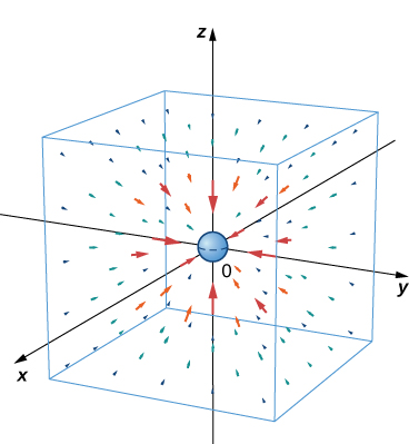
The mass of asteroid 1 is 750,000 kg and the mass of asteroid 2 is 130,000 kg. Assume asteroid 1 is located at the origin, and asteroid 2 is located at \((15,-5,10),\) measured in units of 10 to the eighth power kilometers. Given that the universal gravitational constant is \(G=6.67384\,\times \,{10}^{-11}{\,\text{m}}^{3}{\text{kg}}^{-1}{\text{s}}^{-2},\) find the gravitational force vector that asteroid 1 exerts on asteroid 2.
\(-1.49063\,\times \,{10}^{-18},4.96876\,\times \,{10}^{-19},-9.93752\,\times \,{10}^{-19}\text{N}\)
Gradient Fields
In this section, we study a special kind of vector field called a gradient field or a conservative field. These vector fields are extremely important in physics because they can be used to model physical systems in which energy is conserved. Gravitational fields and electric fields associated with a static charge are examples of gradient fields.
Recall that if \(f\) is a (scalar) function of x and y, then the gradient of \(f\) is
\[\text{grad}\,f=\nabla f={f}_{x}(x,y)\text{i}+{f}_{y}(x,y)\text{j}.\]
We can see from the form in which the gradient is written that \(\nabla f\) is a vector field in \({ℝ}^{2}.\) Similarly, if \(f\) is a function of x, y, and z, then the gradient of \(f\) is
\[\text{grad}\,f=\nabla f={f}_{x}(x,y,z)\text{i}+{f}_{y}(x,y,z)\text{j}+{f}_{z}(x,y,z)\text{k}.\]
The gradient of a three-variable function is a vector field in \({ℝ}^{3}.\)
A gradient field is a vector field that can be written as the gradient of a function, and we have the following definition.
A vector field \(\text{F}\) in \({ℝ}^{2}\) or in \({ℝ}^{3}\) is a gradient field if there exists a scalar function \(f\) such that \(\nabla f=\text{F}.\)
Use technology to plot the gradient vector field of \(f(x,y)={x}^{2}{y}^{2}.\)
Compute \(\nabla f=\langle f_x,f_y\rangle\) first, then let software plot the resulting field.
The gradient of \(f\) is \(\nabla f=\langle 2x{y}^{2},2{x}^{2}y\rangle .\) To sketch the vector field, use a computer algebra system such as Mathematica. Figure 8 shows \(\nabla f.\)
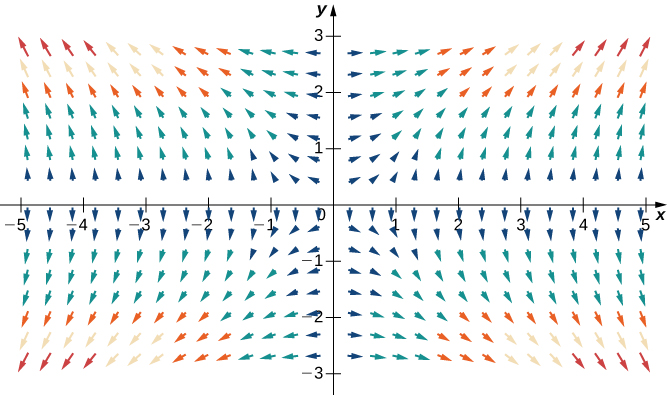
Use technology to plot the gradient vector field of \(f(x,y)=\text{sin}\,x\,\text{cos}\,y.\)
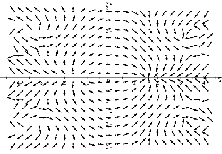
Consider the function \(f(x,y)={x}^{2}{y}^{2}\) from Example 9. Figure 10 shows the level curves of this function overlaid on the function’s gradient vector field. The gradient vectors are perpendicular to the level curves, and the magnitudes of the vectors get larger as the level curves get closer together, because closely grouped level curves indicate the graph is steep, and the magnitude of the gradient vector is the largest value of the directional derivative. Therefore, you can see the local steepness of a graph by investigating the corresponding function’s gradient field.
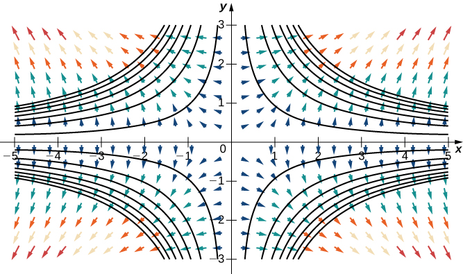
As we learned earlier, a vector field \(\text{F}\) is a conservative vector field, or a gradient field if there exists a scalar function \(f\) such that \(\nabla f=\text{F}.\) In this situation, \(f\) is called a potential function for \(\text{F}.\) Conservative vector fields arise in many applications, particularly in physics. The reason such fields are called conservative is that they model forces of physical systems in which energy is conserved. We study conservative vector fields in more detail later in this chapter.
You might notice that, in some applications, a potential function \(f\) for F is defined instead as a function such that \(\text{-}\nabla f=\text{F}.\) This is the case for certain contexts in physics, for example.
Is \(f(x,y,z)={x}^{2}yz-\text{sin}(xy)\) a potential function for vector field
\[\text{F}(x,y,z)=\langle 2xyz-y\,\text{cos}(xy),{x}^{2}z-x\,\text{cos}(xy),{x}^{2}y\rangle ?\]
Compute the three partial derivatives \(f_x, f_y, f_z\) and compare them to the components of \(\text{F}.\)
We need to confirm whether \(\nabla f=\text{F}.\) We have
\[{f}_{x}=2xyz-y\,\text{cos}(xy),{f}_{y}={x}^{2}z-x\,\text{cos}(xy),\,\text{and}\,{f}_{z}={x}^{2}y.\]
Therefore, \(\nabla f=\text{F}\) and \(f\) is a potential function for \(\text{F}.\)
Is \(f(x,y,z)={x}^{2}\text{cos}(yz)+{y}^{2}{z}^{2}\) a potential function for \(\text{F}(x,y,z)=\langle 2x\,\text{cos}(yz),\text{-}{x}^{2}z\,\text{sin}(yz)+2y{z}^{2},{y}^{2}\rangle ?\)
No
The velocity of a fluid is modeled by field \(\text{v}(x,y)=\langle xy,\frac{{x}^{2}}{2}-y\rangle .\) Verify that \(f(x,y)=\frac{{x}^{2}y}{2}-\frac{{y}^{2}}{2}\) is a potential function for v.
Compute \(f_x\) and \(f_y\) and check they match the components of \(\text{v}.\)
To show that \(f\) is a potential function, we must show that \(\nabla f=\text{v}.\) Note that \({f}_{x}=xy\) and \({f}_{y}=\frac{{x}^{2}}{2}-y.\) Therefore, \(\nabla f=\langle xy,\frac{{x}^{2}}{2}-y\rangle\) and \(f\) is a potential function for v (Figure 10).
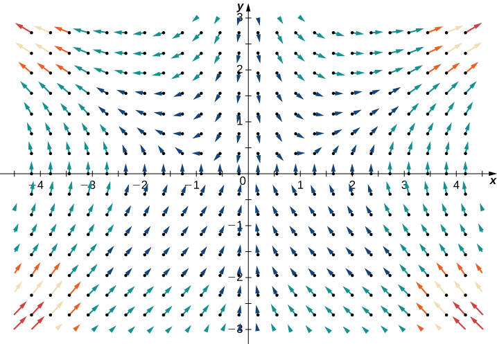
Verify that \(f(x,y)={x}^{3}{y}^{2}+1\) is a potential function for velocity field \(\text{v}(x,y)=⟨3{x}^{2}{y}^{2},2{x}^{3}y⟩.\)
\(\nabla f=\text{v}\)
If F is a conservative vector field, then there is at least one potential function \(f\) such that \(\nabla f=\text{F}.\) But, could there be more than one potential function? If so, is there any relationship between two potential functions for the same vector field? Before answering these questions, let’s recall some facts from single-variable calculus to guide our intuition. Recall that if \(k(x)\) is an integrable function, then k has infinitely many antiderivatives. Furthermore, if F and G are both antiderivatives of k, then F and G differ only by a constant. That is, there is some number C such that \(F(x)=G(x)+C.\)
Now let \(F\) be a conservative vector field and let \(f\) and g be potential functions for \(F\) . Since the gradient is like a derivative, \(F\) being conservative means that \(F\) is “integrable” with “antiderivatives” \(f\) and g. Therefore, if the analogy with single-variable calculus is valid, we expect there is some constant C such that \(f(x)=g(x)+C.\) The next theorem says that this is indeed the case.
To state the next theorem with precision, we need to assume the domain of the vector field is connected and open. To be connected means if \({P}_{1}\) and \({P}_{2}\) are any two points in the domain, then you can walk from \({P}_{1}\) to \({P}_{2}\) along a path that stays entirely inside the domain.
Let F be a conservative vector field on an open and connected domain and let \(f\) and g be functions such that \(\nabla f=\text{F}\) and \(\nabla g=\text{F}.\) Then, there is a constant C such that \(f=g+C.\)
Proof
Since \(f\) and g are both potential functions for F, then \(\nabla (f-g)=\nabla f-\nabla g=\text{F}-\text{F}=0.\) Let \(h=f-g,\) then we have \(\nabla h=0.\) We would like to show that h is a constant function.
Assume h is a function of x and y (the logic of this proof extends to any number of independent variables). Since \(\nabla h=0,\) we have \({h}_{x}=0\) and \({h}_{y}=0.\) The expression \({h}_{x}=0\) implies that h is a constant function with respect to x—that is, \(h(x,y)={k}_{1}(y)\) for some function k1. Similarly, \({h}_{y}=0\) implies \(h(x,y)={k}_{2}(x)\) for some function k2. Therefore, function h depends only on y and also depends only on x. Thus, \(h(x,y)=C\) for some constant C on the connected domain of F. Note that we really do need connectedness at this point; if the domain of F came in two separate pieces, then k could be a constant C1 on one piece but could be a different constant C2 on the other piece. Since \(f-g=h=C,\) we have that \(f=g+C,\) as desired.
□
Conservative vector fields also have a special property called the cross-partial property. This property helps test whether a given vector field is conservative.
Let F be a vector field in two or three dimensions such that the component functions of F have continuous first-order partial derivatives on the domain of F.
If \(\text{F}(x,y)=\langle P(x,y),Q(x,y)\rangle\) is a conservative vector field in \({ℝ}^{2},\) then \(\frac{∂P}{∂y}=\frac{∂Q}{∂x}.\) If \(\text{F}(x,y,z)=\langle P(x,y,z),Q(x,y,z),R(x,y,z)\rangle\) is a conservative vector field in \({ℝ}^{3},\) then
\[\frac{∂P}{∂y}=\frac{∂Q}{∂x},\frac{∂Q}{∂z}=\frac{∂R}{∂y},\,\text{and}\,\frac{∂R}{∂x}=\frac{∂P}{∂z}.\]
Proof
Since F is conservative, there is a function \(f(x,y)\) such that \(\nabla f=\text{F}.\) Therefore, by the definition of the gradient, \({f}_{x}=P\) and \({f}_{y}=Q.\) By Clairaut’s theorem, \({f}_{xy}={f}_{yx},\) But, \({f}_{xy}={P}_{y}\) and \({f}_{yx}={Q}_{x},\) and thus \({P}_{y}={Q}_{x}.\)
□
Clairaut’s theorem gives a fast proof of the cross-partial property of conservative vector fields in \({ℝ}^{3},\) just as it did for vector fields in \({ℝ}^{2}.\)
The Cross-Partial Property of Conservative Vector Fields shows that most vector fields are not conservative. The cross-partial property is difficult to satisfy in general, so most vector fields won’t have equal cross-partials.
Show that rotational vector field \(\text{F}(x,y)=\langle y,\text{-}x\rangle\) is not conservative.
Identify \(P\) and \(Q\), then check whether \(P_y\) equals \(Q_x.\)
Let \(P(x,y)=y\,\text{and}\,Q(x,y)=\text{-}x.\) If F is conservative, then the cross-partials would be equal—that is, \({P}_{y}\) would equal \({Q}_{x.}\) Therefore, to show that F is not conservative, check that \({P}_{y}\ne {Q}_{x}.\) Since \({P}_{y}=1\) and \({Q}_{x}=-1,\) the vector field is not conservative.
Show that the vector field \(\text{F}(x,y)=y\text{i}-{x}^{2}xy\text{j}\) is not conservative.
\({P}_{y}=x\ne {Q}_{x}=-2xy\)
Is vector field \(\text{F}(x,y,z)=\langle 7,-2,{x}^{3}\rangle\) conservative?
Identify \(P, Q, R\) and check all three cross-partial equalities.
Let \(P(x,y,z)=7,\) \(Q(x,y,z)=-2,\) and \(R(x,y,z)={x}^{3}.\) If F is conservative, then all three cross-partial equations will be satisfied—that is, if F is conservative, then \({P}_{y}\) would equal \({Q}_{x},{Q}_{z}\) would equal \({R}_{y},\) and \({R}_{x}\) would equal \({P}_{z}.\) Note that \({P}_{y}={Q}_{x}={R}_{y}={Q}_{z}=0,\) so the first two necessary equalities hold. However, \({R}_{x}=3{x}^{2}\) and \({P}_{z}=0\) so \({R}_{x}\ne {P}_{z}.\) Therefore, \(\text{F}\) is not conservative.
Is vector field \(G(x,y,z)=\langle y,x,xyz\rangle\) conservative?
No
We conclude this section with a word of warning: The Cross-Partial Property of Conservative Vector Fields says that if F is conservative, then F has the cross-partial property. The theorem does not say that, if F has the cross-partial property, then F is conservative (the converse of an implication is not logically equivalent to the original implication). In other words, The Cross-Partial Property of Conservative Vector Fields can only help determine that a field is not conservative; it does not let you conclude that a vector field is conservative. For example, consider vector field \(\text{F}(x,y)=\langle {x}^{2}y,\frac{{x}^{3}}{3}\rangle .\) This field has the cross-partial property, so it is natural to try to use The Cross-Partial Property of Conservative Vector Fields to conclude this vector field is conservative. However, this is a misapplication of the theorem. We learn later how to conclude that F is conservative.
Key Concepts
- A vector field assigns a vector \(\text{F}(x,y)\) to each point \((x,y)\) in a subset D of \({ℝ}^{2}\,\text{or}\,{ℝ}^{3}.\) \(\text{F}(x,y,z)\) to each point \((x,y,z)\) in a subset D of \({ℝ}^{3}.\) (See Example 1.)
- Vector fields can describe the distribution of vector quantities such as forces or velocities over a region of the plane or of space. They are in common use in such areas as physics, engineering, meteorology, oceanography.
- We can sketch a vector field by examining its defining equation to determine relative magnitudes in various locations and then drawing enough vectors to determine a pattern. (See Example 2.)
- A vector field \(\text{F}\) is called conservative if there exists a scalar function \(f\) such that \(\nabla f=\text{F}.\) (See Example 10 and Example 12.)
Key Equations
| Vector field in \({ℝ}^{2}\) | \(\text{F}(x,y)=\langle P(x,y),Q(x,y)\rangle\) or \(\text{F}(x,y)=P(x,y)\text{i}+Q(x,y)\text{j}\) |
| Vector field in \({ℝ}^{3}\) | \(\text{F}(x,y,z)=\langle P(x,y,z),Q(x,y,z),R(x,y,z)\rangle\) or \(\text{F}(x,y,z)=P(x,y,z)\text{i}+Q(x,y,z)\text{j}+R(x,y,z)\text{k}\) |
Section Exercises
The domain of vector field \(\text{F}=\text{F}(x,y)\) is a set of points \((x,y)\) in a plane, and the range of F is a set of what in the plane?
Vectors
For the following exercises, determine whether the statement is true or false.
Vector field \(\text{F}=\langle 3{x}^{2},1\rangle\) is a gradient field for both \({ϕ}_{1}(x,y)={x}^{3}+y\) and \({ϕ}_{2}(x,y)=y+{x}^{3}+100.\)
Vector field \(\text{F}=\frac{\langle y,x\rangle }{\sqrt{{x}^{2}+{y}^{2}}}\) is constant in direction and magnitude on a unit circle.
False
Vector field \(\text{F}=\frac{\langle y,x\rangle }{\sqrt{{x}^{2}+{y}^{2}}}\) is neither a radial field nor a rotation.
For the following exercises, describe each vector field by drawing some of its vectors.
[T] \(\text{F}(x,y)=x\text{i}+y\text{j}\)
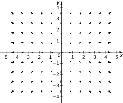
[T] \(\text{F}(x,y)=\text{-}y\text{i}+x\text{j}\)
[T] \(\text{F}(x,y)=x\text{i}-y\text{j}\)
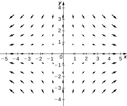
[T] \(\text{F}(x,y)=\text{i}+\text{j}\)
[T] \(\text{F}(x,y)=2x\text{i}+3y\text{j}\)
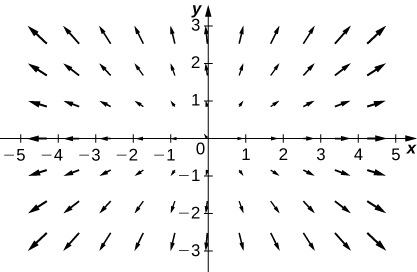
[T] \(\text{F}(x,y)=3\text{i}+x\text{j}\)
[T] \(\text{F}(x,y)=y\text{i}+\text{sin}\,x\text{j}\)
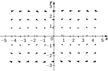
[T] \(\text{F}(x,y,z)=x\text{i}+y\text{j}+z\text{k}\)
[T] \(\text{F}(x,y,z)=2x\text{i}-2y\text{j}-2z\text{k}\)
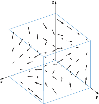
[T] \(\text{F}(x,y,z)=\frac{y}{z}\,\text{i}-\frac{x}{z}\,\text{j}\)
For the following exercises, find the gradient vector field of each function \(f.\)
\(f(x,y)=x\,\text{sin}\,y+\text{cos}\,y\)
\(\text{F}(x,y)=\text{sin}(y)\text{i}+(x\,\text{cos}\,y-\text{sin}\,y)\text{j}\)
\(f(x,y,z)=z{e}^{\text{-}xy}\)
\(f(x,y,z)={x}^{2}y+xy+{y}^{2}z\)
\(\text{F}(x,y,z)=(2xy+y)\text{i}+({x}^{2}+x+2yz)\text{j}+{y}^{2}\text{k}\)
\(f(x,y)={x}^{2}\text{sin}(5y)\)
\(f(x,y)=\text{ln}(1+{x}^{2}+2{y}^{2})\)
\(\text{F}(x,y)=(\frac{2x}{1+{x}^{2}+2{y}^{2}})\text{i}+(\frac{4y}{1+{x}^{2}+2{y}^{2}})\text{j}\)
\(f(x,y,z)=x\,\text{cos}(\frac{y}{z})\)
What is vector field \(\text{F}(x,y)\) with a value at \((x,y)\) that is of unit length and points toward \((1,0)?\)
\(\text{F}(x,y)=\frac{(1-x)\text{i}-y\text{j}}{\sqrt{{(1-x)}^{2}+{y}^{2}}}\)
For the following exercises, write formulas for the vector fields with the given properties.
All vectors are parallel to the x-axis and all vectors on a vertical line have the same magnitude.
All vectors point toward the origin and have constant length.
\(\text{F}(x,y)=\frac{-x\text{i}-y\text{j}}{\sqrt{{x}^{2}+{y}^{2}}}\)
All vectors are of unit length and are perpendicular to the position vector at that point.
Give a formula \(\text{F}(x,y)=M(x,y)\text{i}+N(x,y)\text{j}\) for the vector field in a plane that has the properties that \(\text{F}=0\) at \((0,0)\) and that at any other point \((a,b),\) F is tangent to circle \({x}^{2}+{y}^{2}={a}^{2}+{b}^{2}\) and points in the clockwise direction with magnitude \(\left(F\right)=\sqrt{{a}^{2}+{b}^{2}}.\)
\(\text{F}(x,y)=y\text{i}-x\text{j}\)
Is vector field \(\text{F}(x,y)=\left(P(x,y),Q(x,y)\right)=(\text{sin}\,x+y)\text{i}+(\text{cos}\,y+x)\text{j}\) a gradient field?
Find a formula for vector field \(\text{F}(x,y)=M(x,y)\text{i}+N(x,y)\text{j}\) given the fact that for all points \((x,y),\) F points toward the origin and \(\left(F\right)=\frac{10}{{x}^{2}+{y}^{2}}.\)
\(\text{F}(x,y)=\frac{-10}{{({x}^{2}+{y}^{2})}^{3\text{/}2}}(x\text{i}+y\text{j})\)
For the following exercises, assume that an electric field in the xy-plane caused by an infinite line of charge along the x-axis is a gradient field with potential function \(V(x,y)=c\,\text{ln}(\frac{{r}_{0}}{\sqrt{{x}^{2}+{y}^{2}}}),\) where \(c>0\) is a constant and \({r}_{0}\) is a reference distance at which the potential is assumed to be zero.
Find the components of the electric field in the x- and y-directions, where \(\text{E}(x,y)=\text{-}\nabla V(x,y).\)
Show that the electric field at a point in the xy-plane is directed outward from the origin and has magnitude \(\left(E\right)=\frac{c}{r}\) , where \(r=\sqrt{{x}^{2}+{y}^{2}}\) .
\(\left(E\right)=\frac{c}{{x}^{2}+{y}^{2}}\sqrt{{x}^{2}+{y}^{2}}=\frac{c}{\sqrt{{x}^{2}+{y}^{2}}}=\frac{c}{r}\)
A flow line (or streamline) of a vector field \(\text{F}\) is a curve \(\text{r}(t)\) such that \(d\text{r}\text{/}dt=\text{F}(\text{r}(t)).\) If \(\text{F}\) represents the velocity field of a moving particle, then the flow lines are paths taken by the particle. Therefore, flow lines are tangent to the vector field. For the following exercises, show that the given curve \(\text{c}(t)\) is a flow line of the given velocity vector field \(\text{F}(x,y,z).\)
\(\text{c}(t)=\left({e}^{2t},\text{ln}|t|,\frac{1}{t}\right),t\ne 0;\text{F}(x,y,z)=⟨2x,z,\text{-}{z}^{2}⟩\)
\(\text{c}(t)=\left(\text{sin}\,t,\text{cos}\,t,{e}^{t}\right);\text{F}(x,y,z)=⟨y,\text{-}x,z⟩\)
\(\text{c}\prime (t)=(\text{cos}\,t,\text{-}\text{sin}\,t,{e}^{\text{-}t})=\text{F}(\text{c}(t))\)
For the following exercises, let \(\text{F}=x\text{i}+y\text{j},\) \(\text{G}=\text{-}y\text{i}+x\text{j},\) and \(\text{H}=x\text{i}-y\text{j}.\) Match F, G, and H with their graphs.
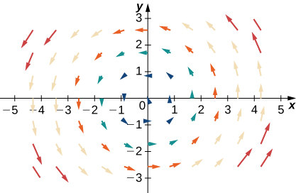
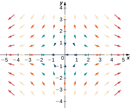
H
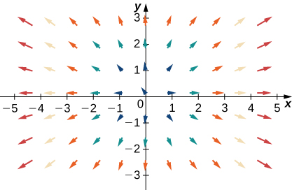
For the following exercises, let \(\text{F}=x\text{i}+y\text{j},\) \(\text{G}=\text{-}y\text{i}+x\text{j},\) and \(\text{H}=x\text{i}-y\text{j}.\) Match the vector fields in a through d with their graphs.
- \(\text{F}+\text{G}\)
- \(\text{F}+\text{H}\)
- \(\text{G}+\text{H}\)
- \(\text{-}\text{F}+\text{G}\)
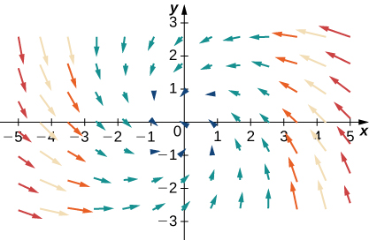
d. \(\text{-}\text{F}+\text{G}\)
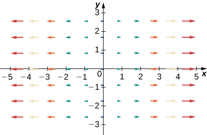
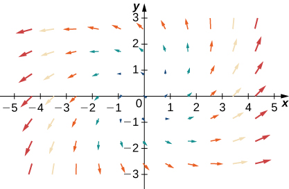
a. \(\text{F}+\text{G}\)
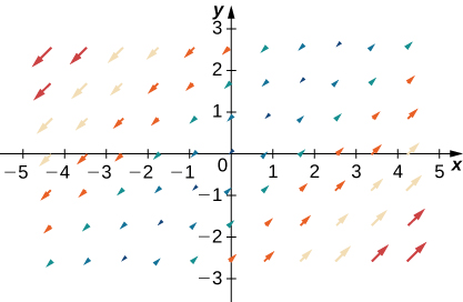
Glossary
- conservative field
- a vector field for which there exists a scalar function \(f\) such that \(\nabla f=\text{F}\)
- gradient field
- a vector field \(\text{F}\) for which there exists a scalar function \(f\) such that \(\nabla f=\text{F};\) in other words, a vector field that is the gradient of a function; such vector fields are also called conservative
- potential function
- a scalar function \(f\) such that \(\nabla f=\text{F}\)
- radial field
- a vector field in which all vectors either point directly toward or directly away from the origin; the magnitude of any vector depends only on its distance from the origin
- rotational field
- a vector field in which the vector at point \((x,y)\) is tangent to a circle with radius \(r=\sqrt{{x}^{2}+{y}^{2}};\) in a rotational field, all vectors flow either clockwise or counterclockwise, and the magnitude of a vector depends only on its distance from the origin
- unit vector field
- a vector field in which the magnitude of every vector is 1
- vector field
- measured in \({ℝ}^{2},\) an assignment of a vector \(\text{F}(x,y)\) to each point \((x,y)\) of a subset \(D\) of \({ℝ}^{2};\) in \({ℝ}^{3},\) an assignment of a vector \(\text{F}(x,y,z)\) to each point \((x,y,z)\) of a subset \(D\) of \({ℝ}^{3}\)