Section 5.7Change of Variables in Multiple Integrals
Recall from Substitution Rule the method of integration by substitution. When evaluating an integral such as \({∫}_{2}^{3}x{({x}^{2}-4)}^{5}dx,\) we substitute \(u=g(x)={x}^{2}-4.\) Then \(du=2x\,dx\) or \(x\,dx=\frac{1}{2}du\) and the limits change to \(u=g(2)={2}^{2}-4=0\) and \(u=g(3)=9-4=5.\) Thus the integral becomes \({∫}_{0}^{5}\frac{1}{2}{u}^{5}du\) and this integral is much simpler to evaluate. In other words, when solving integration problems, we make appropriate substitutions to obtain an integral that becomes much simpler than the original integral.
We also used this idea when we transformed double integrals in rectangular coordinates to polar coordinates and transformed triple integrals in rectangular coordinates to cylindrical or spherical coordinates to make the computations simpler. More generally,
\[\int_{a}^{b}f(x)dx=\int_{c}^{d}f(g(u))g\prime (u)du,\]
Where \(x=g(u),dx=g\prime (u)du,\) and \(u=c\) and \(u=d\) satisfy \(c={g}^{-1}(a)\) and \(d={g}^{-1}(b).\)
A similar result occurs in double integrals when we substitute \(x=h(r,θ)=r\,\text{cos}\,θ,\) \(y=g(r,θ)=r\,\text{sin}\,θ,\) and \(dA=dx\,dy=r\,dr\,dθ.\) Then we get
\[\underset{R}{∬}f(x,y)dA=\underset{S}{∬}f(r\,\text{cos}\,θ,r\,\text{sin}\,θ)r\,dr\,dθ\]
where the domain \(R\) is replaced by the domain \(S\) in polar coordinates. Generally, the function that we use to change the variables to make the integration simpler is called a transformation or mapping.
Planar Transformations
A planar transformation \(T\) is a function that transforms a region \(G\) in one plane into a region \(R\) in another plane by a change of variables. Both \(G\) and \(R\) are subsets of \({ℝ}^{2}.\) For example, Figure 1 shows a region \(G\) in the \(uv\text{-plane}\) transformed into a region \(R\) in the \(xy\text{-plane}\) by the change of variables \(x=g(u,v)\) and \(y=h(u,v),\) or sometimes we write \(x=x(u,v)\) and \(y=y(u,v).\) We shall typically assume that each of these functions has continuous first partial derivatives, which means \({g}_{u},{g}_{v},{h}_{u},\) and \({h}_{v}\) exist and are also continuous. The need for this requirement will become clear soon.
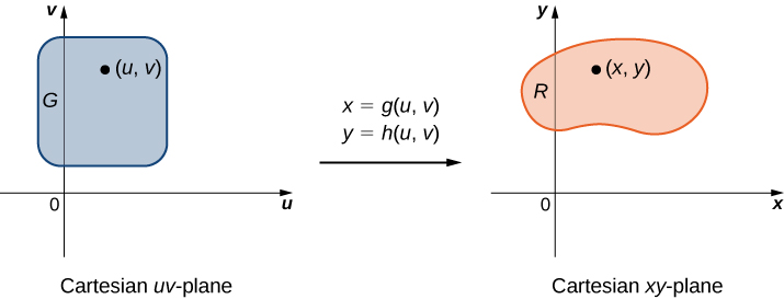
A transformation \(T\text{:}\,G\to R,\) defined as \(T(u,v)=(x,y),\) is said to be a one-to-one transformation if no two points map to the same image point.
To show that \(T\) is a one-to-one transformation, we assume \(T({u}_{1},{v}_{1})=T({u}_{2},{v}_{2})\) and show that as a consequence we obtain \(({u}_{1},{v}_{1})=({u}_{2},{v}_{2}).\) If the transformation \(T\) is one-to-one in the domain \(G,\) then the inverse \({T}^{-1}\) exists with the domain \(R\) such that \({T}^{-1}∘T\) and \(T∘{T}^{-1}\) are identity functions.
Figure 1 shows the mapping \(T(u,v)=(x,y)\) where \(x\) and \(y\) are related to \(u\) and \(v\) by the equations \(x=g(u,v)\) and \(y=h(u,v).\) The region \(G\) is the domain of \(T\) and the region \(R\) is the range of \(T,\) also known as the image of \(G\) under the transformation \(T.\)
Suppose a transformation \(T\) is defined as \(T(r,θ)=(x,y)\) where \(x=r\,\text{cos}\,θ,y=r\,\text{sin}\,θ.\) Find the image of the polar rectangle \(G=\{(r,θ)|0<r\le 1,0\le θ\le \pi \text{/}2\}\) in the \(rθ\text{-plane}\) to a region \(R\) in the \(xy\text{-plane}\text{.}\) Show that \(T\) is a one-to-one transformation in \(G\) and find \({T}^{-1}(x,y).\)
Track how the r and θ bounds map to x,y bounds, then assume T(r1,θ1)=T(r2,θ2) to prove the transformation is one-to-one.
Since \(r\) varies from 0 to 1 in the \(rθ\text{-plane},\) we have a circular disc of radius 0 to 1 in the \(xy\text{-plane}\text{.}\) Because \(θ\) varies from 0 to \(\pi \text{/2}\) in the \(rθ\text{-plane},\) we end up getting a quarter circle of radius \(1\) in the first quadrant of the \(xy\text{-plane}\) (Figure 2). Hence \(R\) is a quarter circle bounded by \({x}^{2}+{y}^{2}=1\) in the first quadrant.
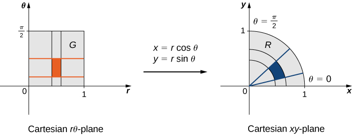
In order to show that \(T\) is a one-to-one transformation, assume \(T({r}_{1},{θ}_{1})=T({r}_{2},{θ}_{2})\) and show as a consequence that \(({r}_{1},{θ}_{1})=({r}_{2},{θ}_{2}).\) In this case, we have
\[\begin{array}{lll}T({r}_{1},{θ}_{1}) & = & T({r}_{2},{θ}_{2}), \\ ({x}_{1},{y}_{1}) & = & ({x}_{2},{y}_{2}), \\ ({r}_{1}\text{cos}\,{θ}_{1},{r}_{1}\text{sin}\,{θ}_{1}) & = & ({r}_{2}\text{cos}\,{θ}_{2},{r}_{2}\text{sin}\,{θ}_{2}), \\ {r}_{1}\text{cos}\,{θ}_{1} & = & {r}_{2}\text{cos}\,{θ}_{2} \\ {r}_{1}\text{sin}\,{θ}_{1} & = & {r}_{2}\text{sin}\,{θ}_{2}\end{array}\]
Dividing, we obtain
\[\begin{array}{lll}\frac{{r}_{1}\text{cos}\,{θ}_{1}}{{r}_{1}\text{sin}\,{θ}_{1}} & = & \frac{{r}_{2}\text{cos}\,{θ}_{2}}{{r}_{2}\text{sin}\,{θ}_{2}} \\ \frac{\text{cos}\,{θ}_{1}}{\text{sin}\,{θ}_{1}} & = & \frac{\text{cos}\,{θ}_{2}}{\text{sin}\,{θ}_{2}} \\ \text{cot}\,{θ}_{1} & = & \text{cot}\,{θ}_{2} \\ {θ}_{1} & = & {θ}_{2}\end{array}\]
since the cotangent function is one-one function in the interval \(0\le θ\le \pi \text{/}2.\) Also, since \(0<r\le 1,\) we have \({r}_{1}={r}_{2},{θ}_{1}={θ}_{2}.\) Therefore, \(({r}_{1},{θ}_{1})=({r}_{2},{θ}_{2})\) and \(T\) is a one-to-one transformation from \(G\) into \(R.\)
To find \({T}^{-1}(x,y)\) solve for \(r,θ\) in terms of \(x,y.\) We already know that \({r}^{2}={x}^{2}+{y}^{2}\) and \(\text{tan}\,θ=\frac{y}{x}.\) Thus \({T}^{-1}(x,y)=(r,θ)\) is defined as \(r=\sqrt{{x}^{2}+{y}^{2}}\) and \(θ={\text{tan}}^{-1}(\frac{y}{x}).\)
Let the transformation \(T\) be defined by \(T(u,v)=(x,y)\) where \(x={u}^{2}-{v}^{2}\) and \(y=uv.\) Find the image of the triangle in the \(uv\text{-plane}\) with vertices \((0,0),(0,1),\) and \((1,1).\)
Trace each of the triangle's three sides through the transformation one at a time to see what curve each one becomes.
The triangle and its image are shown in Figure 3. To understand how the sides of the triangle transform, call the side that joins \((0,0)\) and \((0,1)\) side \(A,\) the side that joins \((0,0)\) and \((1,1)\) side \(B,\) and the side that joins \((1,1)\) and \((0,1)\) side \(C.\)
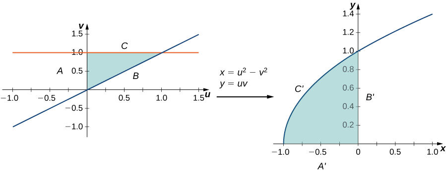
For the side \(A\text{:}\,u=0,0\le v\le 1\) transforms to \(x=\text{-}{v}^{2},y=0\) so this is the side \(A\prime\) that joins \((-1,0)\) and \((0,0).\)
For the side \(B\text{:}\,u=v,0\le u\le 1\) transforms to \(x=0,y={u}^{2}\) so this is the side \({B}^{\prime }\) that joins \((0,0)\) and \((0,1).\)
For the side \(C\text{:}\,0\le u\le 1,v=1\) transforms to \(x={u}^{2}-1,y=u\) (hence \(x={y}^{2}-1)\) so this is the side \({C}^{\prime }\) that makes the upper half of the parabolic arc joining \((-1,0)\) and \((0,1).\)
All the points in the entire region of the triangle in the \(uv\text{-plane}\) are mapped inside the parabolic region in the \(xy\text{-plane}\text{.}\)
Let a transformation \(T\) be defined as \(T(u,v)=(x,y)\) where \(x=u+v,y=3v.\) Find the image of the rectangle \(G=\{(u,v)\text{:}\,0\le u\le 1,0\le v\le 2\}\) from the \(uv\text{-plane}\) after the transformation into a region \(R\) in the \(xy\text{-plane}\text{.}\) Show that \(T\) is a one-to-one transformation and find \({T}^{-1}(x,y).\)
\({T}^{-1}(x,y)=(u,v)\) where \(u=\frac{3x-y}{3}\) and \(v=\frac{y}{3}\)
Jacobians
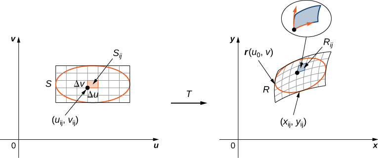
Recall that we mentioned near the beginning of this section that each of the component functions must have continuous first partial derivatives, which means that \({g}_{u},{g}_{v},{h}_{u},\) and \({h}_{v}\) exist and are also continuous. A transformation that has this property is called a \({C}^{1}\) transformation (here \(C\) denotes continuous). Let \(T(u,v)=(g(u,v),h(u,v)),\) where \(x=g(u,v)\) and \(y=h(u,v),\) be a one-to-one \({C}^{1}\) transformation. We want to see how it transforms a small rectangular region \(S,\) \(\Delta u\) units by \(\Delta v\) units, in the \(uv\text{-plane}\) (see the following figure).
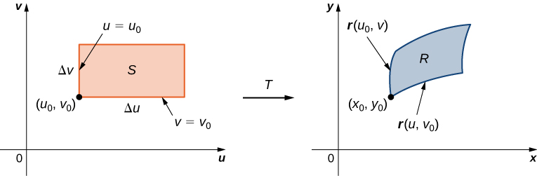
Since \(x=g(u,v)\) and \(y=h(u,v),\) we have the position vector \(r(u,v)=g(u,v)i+h(u,v)j\) of the image of the point \((u,v).\) Suppose that \(({u}_{0},{v}_{0})\) is the coordinate of the point at the lower left corner that mapped to \(({x}_{0},{y}_{0})=T({u}_{0},{v}_{0}).\) The line \(v={v}_{0}\) maps to the image curve with vector function \(\text{r}(u,{v}_{0}),\) and the tangent vector at \(({x}_{0},{y}_{0})\) to the image curve is
\[{r}_{u}={g}_{u}({u}_{0},{v}_{0})i+{h}_{u}({u}_{0},{v}_{0})j=\frac{∂x}{∂u}i+\frac{∂y}{∂u}j.\]
Similarly, the line \(u={u}_{0}\) maps to the image curve with vector function \(r({u}_{0},v),\) and the tangent vector at \(({x}_{0},{y}_{0})\) to the image curve is
\[{r}_{v}={g}_{v}({u}_{0},{v}_{0})i+{h}_{v}({u}_{0},{v}_{0})j=\frac{∂x}{∂v}i+\frac{∂y}{∂v}j.\]
Now, note that
\[{r}_{u}=\underset{\Delta u\to 0}{\text{lim}}\frac{r({u}_{0}+\Delta u,{v}_{0})-r({u}_{0},{v}_{0})}{\Delta u}\,\text{so}\,r({u}_{0}+\Delta u,{v}_{0})-r({u}_{0},{v}_{0})\approx \Delta u{r}_{u}.\]
Similarly,
\[{r}_{v}=\underset{\Delta v\to 0}{\text{lim}}\frac{r({u}_{0},{v}_{0}+\Delta v)-r({u}_{0},{v}_{0})}{\Delta v}\,\text{so}\,r({u}_{0},{v}_{0}+\Delta v)-r({u}_{0},{v}_{0})\approx \Delta v{r}_{v}.\]
This allows us to estimate the area \(\Delta A\) of the image \(R\) by finding the area of the parallelogram formed by the sides \(\Delta v{r}_{v}\) and \(\Delta u{r}_{u}.\) By using the cross product of these two vectors by adding the k component as \(0,\) the area \(\Delta A\) of the image \(R\) (refer to The Cross Product) is approximately \(||\Delta {ur}_{u}\,\times \,\Delta {vr}_{v}||=||{r}_{u}\,\times \,{r}_{v}||\Delta u\Delta v.\) In determinant form, the cross product is
\[{r}_{u}\,\times \,{r}_{v}=|\begin{array}{lllll}i & & j & & k \\ \frac{∂x}{∂u} & & \frac{∂y}{∂u} & & 0 \\ \frac{∂x}{∂v} & & \frac{∂y}{∂v} & & 0\end{array}|=|\begin{array}{lll}\frac{∂x}{∂u} & & \frac{∂y}{∂u} \\ \frac{∂x}{∂v} & & \frac{∂y}{∂v}\end{array}|k=(\frac{∂x}{∂u}\,\frac{∂y}{∂v}-\frac{∂x}{∂v}\,\frac{∂y}{∂u})k.\]
Since \(||k||=1,\) we have \(\Delta A\approx ||{r}_{u}\,\times \,{r}_{v}||\Delta u\Delta v=(\frac{∂x}{∂u}\,\frac{∂y}{∂v}-\frac{∂x}{∂v}\,\frac{∂y}{∂u})\Delta u\Delta v.\)
The Jacobian of the \({C}^{1}\) transformation \(T(u,v)=(g(u,v),h(u,v))\) is denoted by \(J(u,v)\) and is defined by the \(2\,\times \,2\) determinant
\[J(u,v)=|\frac{∂(x,y)}{∂(u,v)}|=|\begin{array}{lll}\frac{∂x}{∂u} & & \frac{∂y}{∂u} \\ \frac{∂x}{∂v} & & \frac{∂y}{∂v}\end{array}|=(\frac{∂x}{∂u}\,\frac{∂y}{∂v}-\frac{∂x}{∂v}\,\frac{∂y}{∂u}).\]
Using the definition, we have
\[\Delta A\approx J(u,v)\Delta u\Delta v=|\frac{∂(x,y)}{∂(u,v)}|\Delta u\Delta v.\]
Note that the Jacobian is frequently denoted simply by
\[J(u,v)=\frac{∂(x,y)}{∂(u,v)}.\]
Note also that
\[|\begin{array}{lll}\frac{∂x}{∂u} & & \frac{∂y}{∂u} \\ \frac{∂x}{∂v} & & \frac{∂y}{∂v}\end{array}|=(\frac{∂x}{∂u}\,\frac{∂y}{∂v}-\frac{∂x}{∂v}\,\frac{∂y}{∂u})=|\begin{array}{lll}\frac{∂x}{∂u} & & \frac{∂x}{∂v} \\ \frac{∂y}{∂u} & & \frac{∂y}{∂v}\end{array}|.\]
Hence the notation \(J(u,v)=\frac{∂(x,y)}{∂(u,v)}\) suggests that we can write the Jacobian determinant with partials of \(x\) in the first row and partials of \(y\) in the second row.
Find the Jacobian of the transformation given in Example 1.
Compute the four partial derivatives of x and y with respect to r and θ, then evaluate the resulting 2×2 determinant.
The transformation in the example is \(T(r,θ)=(r\,\text{cos}\,θ,r\,\text{sin}\,θ)\) where \(x=r\,\text{cos}\,θ\) and \(y=r\,\text{sin}\,θ.\) Thus the Jacobian is
\[\begin{array}{ll}J(r,θ) & =\frac{∂(x,y)}{∂(r,θ)}=|\begin{array}{lll}\frac{∂x}{∂r} & & \frac{∂x}{∂θ} \\ \frac{∂y}{∂r} & & \frac{∂y}{∂θ}\end{array}|=|\begin{array}{lll}\text{cos}\,θ & & -r\,\text{sin}\,θ \\ \text{sin}\,θ & & r\,\text{cos}\,θ\end{array}| \\ & =r\,{\text{cos}}^{2}θ+r\,{\text{sin}}^{2}θ=r({\text{cos}}^{2}θ+{\text{sin}}^{2}θ)=r.\end{array}\]
Find the Jacobian of the transformation given in Example 2.
Take the partial derivatives of x=u²-v² and y=uv, then form the 2×2 Jacobian determinant.
The transformation in the example is \(T(u,v)=({u}^{2}-{v}^{2},uv)\) where \(x={u}^{2}-{v}^{2}\) and \(y=uv.\) Thus the Jacobian is
\[J(u,v)=\frac{∂(x,y)}{∂(u,v)}=|\begin{array}{lll}\frac{∂x}{∂u} & & \frac{∂x}{∂v} \\ \frac{∂y}{∂u} & & \frac{∂y}{∂v}\end{array}|=|\begin{array}{lll}2u & & v \\ -2v & & u\end{array}|=2{u}^{2}+2{v}^{2}.\]
Find the Jacobian of the transformation: \(T(u,v)=(u+v,2v).\)
\(J(u,v)=\frac{∂(x,y)}{∂(u,v)}=|\begin{array}{lll}\frac{∂x}{∂u} & & \frac{∂x}{∂v} \\ \frac{∂y}{∂u} & & \frac{∂y}{∂v}\end{array}|=|\begin{array}{lll}1 & & 1 \\ 0 & & 2\end{array}|=2\)
Change of Variables for Double Integrals
We have already seen that, under the change of variables \(T(u,v)=(x,y)\) where \(x=g(u,v)\) and \(y=h(u,v),\) a small region \(\Delta A\) in the \(xy\text{-plane}\) is related to the area formed by the product \(\Delta u\Delta v\) in the \(uv\text{-plane}\) by the approximation
\[\Delta A\approx J(u,v)\Delta u,\Delta v.\]
Now let’s go back to the definition of double integral for a minute:
\[\underset{R}{∬}f(x,y)dA=\underset{m,n\to \infty }{\text{lim}}\sum_{i=1}^{m}\sum_{j=1}^{n}f({x}_{ij},{y}_{ij})\Delta A.\]
Referring to Figure 5, observe that we divided the region \(S\) in the \(uv\text{-plane}\) into small subrectangles \({S}_{ij}\) and we let the subrectangles \({R}_{ij}\) in the \(xy\text{-plane}\) be the images of \({S}_{ij}\) under the transformation \(T(u,v)=(x,y).\)
Then the double integral becomes
\[\underset{R}{∬}f(x,y)dA=\underset{m,n\to \infty }{\text{lim}}\sum_{i=1}^{m}\sum_{j=1}^{n}f({x}_{ij},{y}_{ij})\Delta A=\underset{m,n\to \infty }{\text{lim}}\sum_{i=1}^{m}\sum_{j=1}^{n}f(g({u}_{ij},{v}_{ij}),h({u}_{ij},{v}_{ij}))|J({u}_{ij},{v}_{ij})|\Delta u\Delta v.\]
Notice this is exactly the double Riemann sum for the integral
\[\underset{S}{∬}f(g(u,v),h(u,v))|\frac{∂(x,y)}{∂(u,v)}|du\,dv.\]
Let \(T(u,v)=(x,y)\) where \(x=g(u,v)\) and \(y=h(u,v)\) be a one-to-one \({C}^{1}\) transformation, with a nonzero Jacobian on the interior of the region \(S\) in the \(uv\text{-plane;}\) it maps \(S\) into the region \(R\) in the \(xy\text{-plane}\text{.}\) If \(f\) is continuous on \(R,\) then
\[\underset{R}{∬}f(x,y)dA=\underset{S}{∬}f(g(u,v),h(u,v))|\frac{∂(x,y)}{∂(u,v)}|du\,dv.\]
With this theorem for double integrals, we can change the variables from \((x,y)\) to \((u,v)\) in a double integral simply by replacing
\[dA=dx\,dy=|\frac{∂(x,y)}{∂(u,v)}|du\,dv\]
when we use the substitutions \(x=g(u,v)\) and \(y=h(u,v)\) and then change the limits of integration accordingly. This change of variables often makes any computations much simpler.
Consider the integral
\[\int_{0}^{2}\,\int_{0}^{\sqrt{2x-{x}^{2}}}\sqrt{{x}^{2}+{y}^{2}}\,dy\,dx.\]
Use the change of variables \(x=r\,\text{cos}\,θ\) and \(y=r\,\text{sin}\,θ,\) and find the resulting integral.
Identify the region as the upper half of a circle, rewrite its boundary in polar form, then substitute the Jacobian r for dA.
First we need to find the region of integration. This region is bounded below by \(y=0\) and above by \(y=\sqrt{2x-{x}^{2}}\) (see the following figure).
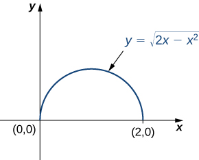
Squaring and collecting terms, we find that the region is the upper half of the circle \({x}^{2}+{y}^{2}-2x=0,\) that is, \({y}^{2}+{(x-1)}^{2}=1.\) In polar coordinates, the circle is \(r=2\,\text{cos}\,θ\) so the region of integration in polar coordinates is bounded by \(0\le r\le 2 \text{cos}\,θ\) and \(0\le θ\le \frac{\pi }{2}.\)
The Jacobian is \(J(r,θ)=r,\) as shown in Example 3. Since \(r\ge 0,\) we have \(|J(r,θ)|=r.\)
The integrand \(\sqrt{{x}^{2}+{y}^{2}}\) changes to \(r\) in polar coordinates, so the double iterated integral is
\[\int_{0}^{2}\,\int_{0}^{\sqrt{2x-{x}^{2}}}\sqrt{{x}^{2}+{y}^{2}}dy\,dx=\int_{0}^{\pi \text{/}2}\,\int_{0}^{2\,\text{cos}\,θ}r|J(r,θ)|dr\,dθ=\int_{0}^{\pi \text{/}2}\,\int_{0}^{2\,\text{cos}\,θ}{r}^{2}dr\,dθ.\]
Considering the integral \(\int_{0}^{1}\,\int_{0}^{\sqrt{1-{x}^{2}}}({x}^{2}+{y}^{2})dy\,dx,\) use the change of variables \(x=r\,\text{cos}\,θ\) and \(y=r\,\text{sin}\,θ,\) and find the resulting integral.
\(\int_{0}^{\pi \text{/}2}\,\int_{0}^{1}{r}^{3}dr\,dθ\)
Notice in the next example that the region over which we are to integrate may suggest a suitable transformation for the integration. This is a common and important situation.
Consider the integral \(\underset{R}{∬}(x-y)dy\,dx,\) where \(R\) is the parallelogram joining the points \((1,2),\) \((3,4),(4,3),\) and \((6,5)\) (Figure 7). Make appropriate changes of variables, and write the resulting integral.
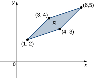
Notice the parallelogram's sides are level curves of x-y and x-3y, so let u=x-y and v=x-3y to straighten the region into a rectangle.
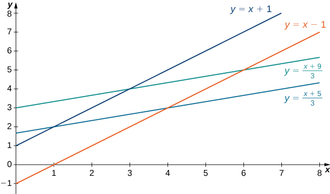
First, we need to understand the region over which we are to integrate. The sides of the parallelogram are \(x-y+1=0,x-y-1=0,\) \(x-3y+5=0,\text{and}\,x-3y+9=0\) (Figure 8). Another way to look at them is \(x-y=-1,x-y=1,\) \(x-3y=-5,\) and \(x-3y=-9.\)
Clearly the parallelogram is bounded by the lines \(y=x+1,y=x-1,y=\frac{1}{3}(x+5),\) and \(y=\frac{1}{3}(x+9).\)
Notice that if we were to make \(u=x-y\) and \(v=x-3y,\) then the limits on the integral would be \(-1\le u\le 1\) and \(-9\le v\le -5.\)
To solve for \(x\) and \(y,\) we multiply the first equation by \(3\) and subtract the second equation, \(3u-v=(3x-3y)-(x-3y)=2x.\) Then we have \(x=\frac{3u-v}{2}.\) Moreover, if we simply subtract the second equation from the first, we get \(u-v=(x-y)-(x-3y)=2y\) and \(y=\frac{u-v}{2}.\)
Thus, we can choose the transformation
\[T(u,v)=(\frac{3u-v}{2},\frac{u-v}{2})\]
and compute the Jacobian \(J(u,v).\) We have
\[J(u,v)=\frac{∂(x,y)}{∂(u,v)}=|\begin{array}{lll}\frac{∂x}{∂u} & & \frac{∂x}{∂v} \\ \frac{∂y}{∂u} & & \frac{∂y}{∂v}\end{array}|=|\begin{array}{lll}3\text{/}2 & & -1\text{/}2 \\ 1\text{/}2 & & -1\text{/}2\end{array}|=-\frac{3}{4}+\frac{1}{4}=-\frac{1}{2}.\]
Therefore, \(|J(u,v)|=\frac{1}{2}.\) Also, the original integrand becomes
\[x-y=\frac{1}{2}[3u-v-u+v]=\frac{1}{2}[3u-u]=\frac{1}{2}[2u]=u.\]
Therefore, by the use of the transformation \(T,\) the integral changes to
\[\underset{R}{∬}(x-y)dy\,dx=\int_{-9}^{-5}\,\int_{-1}^{1}J(u,v)u\,du\,dv=\int_{-9}^{-5}\,\int_{-1}^{1}(\frac{1}{2})u\,du\,dv,\]
which is much simpler to compute. In fact, it is easily found to be zero. And this is just one example of why we transform integrals like this.
Make appropriate changes of variables in the integral \(\underset{R}{∬}\frac{4}{{(x-y)}^{2}}dy\,dx,\) where \(R\) is the trapezoid bounded by the lines \(x-y=2,x-y=4,x=0,\text{and}\,y=0.\) Write the resulting integral.
\(x=\frac{1}{2}(v+u)\) and \(y=\frac{1}{2}(v-u)\) and \(\int_{2}^{4}\,\int_{-u}^{u}\frac{4}{{u}^{2}}(\frac{1}{2})dv\,du.\)
We are ready to give a problem-solving strategy for change of variables.
- Sketch the region given by the problem in the \(xy\text{-plane}\) and then write the equations of the curves that form the boundary.
- Depending on the region or the integrand, choose the transformations \(x=g(u,v)\) and \(y=h(u,v).\)
- Determine the new limits of integration in the \(uv\text{-plane}\text{.}\)
- Find the Jacobian \(J(u,v).\)
- In the integrand, replace the variables to obtain the new integrand.
- Replace \(dy\,dx\) or \(dx\,dy,\) whichever occurs, by \(J(u,v)du\,dv.\)
In the next example, we find a substitution that makes the integrand much simpler to compute.
Using the change of variables \(u=x-y\) and \(v=x+y,\) evaluate the integral
\[\underset{R}{∬}(x-y){e}^{{x}^{2}-{y}^{2}}dA,\]
where \(R\) is the region bounded by the lines \(x+y=1\) and \(x+y=3\) and the curves \({x}^{2}-{y}^{2}=-1\) and \({x}^{2}-{y}^{2}=1\) (see the first region in Figure 9).
Rewrite the boundary curves in terms of u=x-y and v=x+y to turn the curved region into a simple rectangle in the uv-plane.
As before, first find the region \(R\) and picture the transformation so it becomes easier to obtain the limits of integration after the transformations are made (Figure 9).
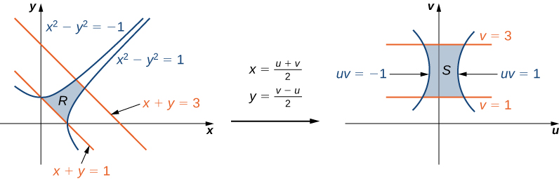
Given \(u=x-y\) and \(v=x+y,\) we have \(x=\frac{u+v}{2}\) and \(y=\frac{v-u}{2}\) and hence the transformation to use is \(T(u,v)=(\frac{u+v}{2},\frac{v-u}{2}).\) The lines \(x+y=1\) and \(x+y=3\) become \(v=1\) and \(v=3,\) respectively. The curves \({x}^{2}-{y}^{2}=1\) and \({x}^{2}-{y}^{2}=-1\) become \(uv=1\) and \(uv=-1,\) respectively.
Thus we can describe the region \(S\) (see the second region Figure 9) as
\[S=\{(u,v)|1\le v\le 3,\frac{-1}{v}\le u\le \frac{1}{v}\}.\]
The Jacobian for this transformation is
\[J(u,v)=\frac{∂(x,y)}{∂(u,v)}=|\begin{array}{lll}\frac{∂x}{∂u} & & \frac{∂x}{∂v} \\ \frac{∂y}{∂u} & & \frac{∂y}{∂v}\end{array}|=|\begin{array}{lll}1\text{/}2 & & -1\text{/}2 \\ 1\text{/}2 & & 1\text{/}2\end{array}|=\frac{1}{2}.\]
Therefore, by using the transformation \(T,\) the integral changes to
\[\underset{R}{∬}(x-y){e}^{{x}^{2}-{y}^{2}}dA=\frac{1}{2}\int_{1}^{3}\,\int_{-1\text{/}v}^{1\text{/}v}u{e}^{uv}du\,dv.\]
Doing the evaluation, we have
\[\frac{1}{2}\int_{1}^{3}\,\int_{-1\text{/}v}^{1\text{/}v}u{e}^{uv}du\,dv=\frac{2}{3e}\approx 0.245.\]
Using the substitutions \(x=v\) and \(y=\sqrt{u+v},\) evaluate the integral \(\underset{R}{∬}y\,\text{sin}({y}^{2}-x)dA\) where \(R\) is the region bounded by the lines \(y=\sqrt{x},x=2,\text{and}\,y=0.\)
\(\frac{1}{2}(\text{sin}\,2-2)\)
Change of Variables for Triple Integrals
Changing variables in triple integrals works in exactly the same way. Cylindrical and spherical coordinate substitutions are special cases of this method, which we demonstrate here.
Suppose that \(G\) is a region in \(uvw\text{-space}\) and is mapped to \(D\) in \(xyz\text{-space}\) (Figure 10) by a one-to-one \({C}^{1}\) transformation \(T(u,v,w)=(x,y,z)\) where \(x=g(u,v,w),\) \(y=h(u,v,w),\) and \(z=k(u,v,w).\)
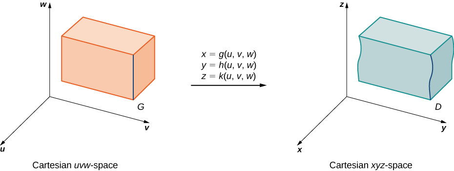
Then any function \(F(x,y,z)\) defined on \(D\) can be thought of as another function \(H(u,v,w)\) that is defined on \(G\text{:}\)
\[F(x,y,z)=F(g(u,v,w),h(u,v,w),k(u,v,w))=H(u,v,w).\]
Now we need to define the Jacobian for three variables.
The Jacobian determinant \(J(u,v,w)\) in three variables is defined as follows:
\[J(u,v,w)=|\begin{array}{lllll}\frac{∂x}{∂u} & & \frac{∂y}{∂u} & & \frac{∂z}{∂u} \\ \frac{∂x}{∂v} & & \frac{∂y}{∂v} & & \frac{∂z}{∂v} \\ \frac{∂x}{∂w} & & \frac{∂y}{∂w} & & \frac{∂z}{∂w}\end{array}|.\]
This is also the same as
\[J(u,v,w)=|\begin{array}{lllll}\frac{∂x}{∂u} & & \frac{∂x}{∂v} & & \frac{∂x}{∂w} \\ \frac{∂y}{∂u} & & \frac{∂y}{∂v} & & \frac{∂y}{∂w} \\ \frac{∂z}{∂u} & & \frac{∂z}{∂v} & & \frac{∂z}{∂w}\end{array}|.\]
The Jacobian can also be simply denoted as \(\frac{∂(x,y,z)}{∂(u,v,w)}.\)
With the transformations and the Jacobian for three variables, we are ready to establish the theorem that describes change of variables for triple integrals.
Let \(T(u,v,w)=(x,y,z)\) where \(x=g(u,v,w),y=h(u,v,w),\) and \(z=k(u,v,w),\) be a one-to-one \({C}^{1}\) transformation, with a nonzero Jacobian, that maps the region \(G\) in the \(uvw\text{-space}\) into the region \(R\) in the \(xyz\text{-space}\text{.}\) As in the two-dimensional case, if \(F\) is continuous on \(R,\) then
\[\begin{array}{ll}\underset{R}{∭}F(x,y,z)dV & =\underset{G}{∭}F(g(u,v,w),h(u,v,w),k(u,v,w))|\frac{∂(x,y,z)}{∂(u,v,w)}|du\,dv\,dw \\ & =\underset{G}{∭}H(u,v,w)|J(u,v,w)|du\,dv\,dw.\end{array}\]
Let us now see how changes in triple integrals for cylindrical and spherical coordinates are affected by this theorem. We expect to obtain the same formulas as in Triple Integrals in Cylindrical and Spherical Coordinates.
Derive the formula in triple integrals for
- cylindrical and
- spherical coordinates.
Write out the 3×3 Jacobian determinant for each transformation and expand it to confirm the r and ρ²sin φ factors.
- For cylindrical coordinates, the transformation is \(T(r,θ,z)=(x,y,z)\) from the Cartesian \(rθz\text{-plane}\) to the Cartesian \(xyz\text{-plane}\) (Figure 11). Here \(x=r\,\text{cos}\,θ,\) \(y=r\,\text{sin}\,θ,\) and \(z=z.\) The Jacobian for the transformation is
We know that \(r\ge 0,\) so \(|J(r,θ,z)|=r.\) Then the triple integral is
\[\begin{array}{ll}J(r,θ,z) & =\frac{∂(x,y,z)}{∂(r,θ,z)}=|\begin{array}{lllll}\frac{∂x}{∂r} & & \frac{∂x}{∂θ} & & \frac{∂x}{∂z} \\ \frac{∂y}{∂r} & & \frac{∂y}{∂θ} & & \frac{∂y}{∂z} \\ \frac{∂z}{∂r} & & \frac{∂z}{∂θ} & & \frac{∂z}{∂z}\end{array}| \\ & =|\begin{array}{lllll}\text{cos}\,θ & & -r\,\text{sin}\,θ & & 0 \\ \text{sin}\,θ & & r\,\text{cos}\,θ & & 0 \\ 0 & & 0 & & 1\end{array}|=r\,{\text{cos}}^{2}θ+r\,{\text{sin}}^{2}θ=r({\text{cos}}^{2}θ+{\text{sin}}^{2}θ)=r.\end{array}\]
\[\underset{D}{∭}f(x,y,z)dV=\underset{G}{∭}f(r\,\text{cos}\,θ,r\,\text{sin}\,θ,z)r\,dr\,dθ\,dz.\]
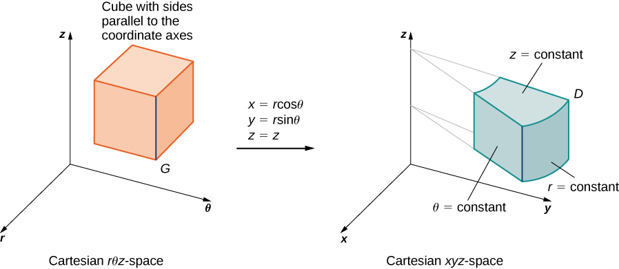
Figure 11 — The transformation from rectangular coordinates to cylindrical coordinates can be treated as a change of variables from region \(G\) in \(rθz\text{-space}\) to region \(D\) in \(xyz\text{-space}.\) - For spherical coordinates, the transformation is \(T(ρ,θ,φ)=(x,y,z)\) from the Cartesian \(pθφ\text{-plane}\) to the Cartesian \(xyz\text{-plane}\) (Figure 12). Here \(x=ρ\,\text{sin}\,φ\,\text{cos}\,θ,\) \(y=ρ\,\text{sin}\,φ\,\text{sin}\,θ,\) and \(z=ρ\,\text{cos}\,φ.\) The Jacobian for the transformation is
Expanding the determinant with respect to the third row:
Since \(0\le φ\le \pi ,\) we must have \(\text{sin}\,φ\ge 0.\) Thus \(|J(ρ,θ,φ)|=|\text{-}{ρ}^{2}\text{sin}\,φ|={ρ}^{2}\text{sin}\,φ.\)
Then the triple integral becomes\[J(ρ,θ,φ)=\frac{∂(x,y,z)}{∂(ρ,θ,φ)}=|\begin{array}{lllll}\frac{∂x}{∂ρ} & & \frac{∂x}{∂θ} & & \frac{∂x}{∂φ} \\ \frac{∂y}{∂ρ} & & \frac{∂y}{∂θ} & & \frac{∂y}{∂φ} \\ \frac{∂z}{∂ρ} & & \frac{∂z}{∂θ} & & \frac{∂z}{∂φ}\end{array}|=|\begin{array}{lllll}\text{sin}\,φ\,\text{cos}\,θ & & ρ\,\text{sin}\,φ\,\text{sin}\,θ & & ρ\,\text{cos}\,φ\,\text{cos}\,θ \\ \text{sin}\,φ\,\text{sin}\,θ & & ρ\,\text{sin}\,φ\,\text{cos}\,θ & & ρ\,\text{cos}\,φ\,\text{sin}\,θ \\ \text{cos}\,ϕ & & 0 & & -ρ\,\text{sin}\,φ\end{array}|.\]
\[\begin{array}{l} \\ \\ =\text{cos}\,φ|\begin{array}{lll}-ρ\,\text{sin}\,φ\,\text{sin}\,θ & & ρ\,\text{cos}\,φ\,\text{cos}\,θ \\ ρ\,\text{sin}\,φ\,\text{sin}\,θ & & ρ\,\text{cos}\,φ\,\text{sin}\,θ\end{array}|-ρ\,\text{sin}\,φ|\begin{array}{lll}\text{sin}\,φ\,\text{cos}\,θ & & -ρ\,\text{sin}\,φ\,\text{sin}\,θ \\ \text{sin}\,φ\,\text{sin}\,θ & & ρ\,\text{sin}\,φ\,\text{cos}\,θ\end{array}| \\ =\text{cos}\,φ(\text{-}{ρ}^{2}\text{sin}\,φ\,\text{cos}\,φ\,{\text{sin}}^{2}θ-{ρ}^{2}\text{sin}\,φ\,\text{cos}\,φ\,{\text{cos}}^{2}θ) \\ \,-ρ\,\text{sin}\,φ(ρ\,{\text{sin}}^{2}φ\,{\text{cos}}^{2}θ+ρ\,{\text{sin}}^{2}φ\,{\text{sin}}^{2}θ) \\ =\text{-}{ρ}^{2}\text{sin}\,φ\,{\text{cos}}^{2}φ({\text{sin}}^{2}θ+{\text{cos}}^{2}θ)-{ρ}^{2}\text{sin}\,φ\,{\text{sin}}^{2}φ({\text{sin}}^{2}θ+{\text{cos}}^{2}θ) \\ =\text{-}{ρ}^{2}\text{sin}\,φ\,{\text{cos}}^{2}φ-{ρ}^{2}\text{sin}\,φ\,{\text{sin}}^{2}φ \\ =\text{-}{ρ}^{2}\text{sin}\,φ({\text{cos}}^{2}φ+{\text{sin}}^{2}φ)=\text{-}{ρ}^{2}\text{sin}\,φ.\end{array}\]
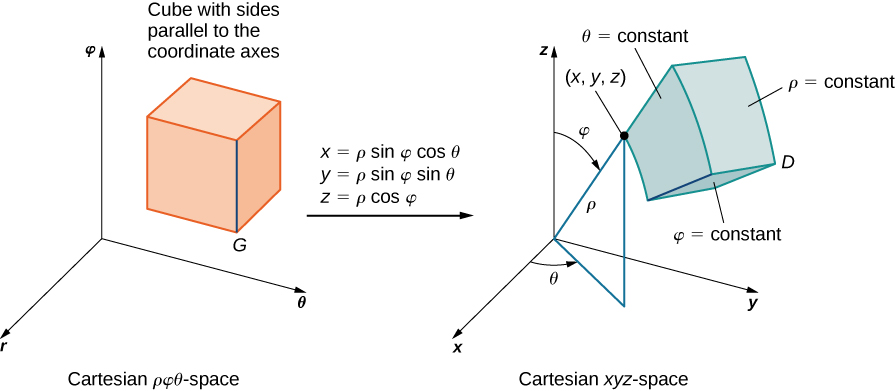
Figure 12 — The transformation from rectangular coordinates to spherical coordinates can be treated as a change of variables from region \(G\) in \(ρθφ\text{-space}\) to region \(D\) in \(xyz\text{-space}\text{.}\) \[\underset{D}{∭}f(x,y,z)dV=\underset{G}{∭}f(ρ\,\text{sin}\,φ\,\text{cos}\,θ,ρ\,\text{sin}\,φ\,\text{sin}\,θ,ρ\,\text{cos}\,φ){ρ}^{2}\text{sin}\,φ\,dρ\,dφ\,dθ.\]
Let’s try another example with a different substitution.
Evaluate the triple integral
\[\int_{0}^{3}\,\int_{0}^{4}\,\int_{y\text{/}2}^{(y\text{/}2)+1}(x+\frac{z}{3})dx\,dy\,dz\]
in \(xyz\text{-space}\) by using the transformation
\[u=(2x-y)\text{/}2,v=y\text{/}2,\text{and}\,w=z\text{/}3.\]
Then integrate over an appropriate region in \(uvw\text{-space}\text{.}\)
Solve the given substitution for x, y, z in terms of u, v, w, then rewrite both the bounds and the integrand in the new variables.
As before, some kind of sketch of the region \(G\) in \(xyz\text{-space}\) over which we have to perform the integration can help identify the region \(D\) in \(uvw\text{-space}\) (Figure 13). Clearly \(G\) in \(xyz\text{-space}\) is bounded by the planes \(x=y\text{/}2,x=(y\text{/}2)+1,y=0,\) \(y=4,\) \(z=0,\text{and}\,z=4.\) We also know that we have to use \(u=(2x-y)\text{/}2,v=y\text{/}2,\text{and}\,w=z\text{/}3\) for the transformations. We need to solve for \(x,y,\text{and}\,z.\) Here we find that \(x=u+v,\) \(y=2v,\) and \(z=3w.\)
Using elementary algebra, we can find the corresponding surfaces for the region \(G\) and the limits of integration in \(uvw\text{-space}\text{.}\) It is convenient to list these equations in a table.
| Equations in \(xyz\) for the region \(D\) | Corresponding equations in \(uvw\) for the region \(G\) | Limits for the integration in \(uvw\) |
| \(x=y\text{/}2\) | \(u+v=2v\text{/}2=v\) | \(u=0\) |
| \(x=y\text{/}2\) | \(u+v=(2v\text{/}2)+1=v+1\) | \(u=1\) |
| \(y=0\) | \(2v=0\) | \(v=0\) |
| \(y=4\) | \(2v=4\) | \(v=2\) |
| \(z=0\) | \(3w=0\) | \(w=0\) |
| \(z=3\) | \(3w=3\) | \(w=1\) |
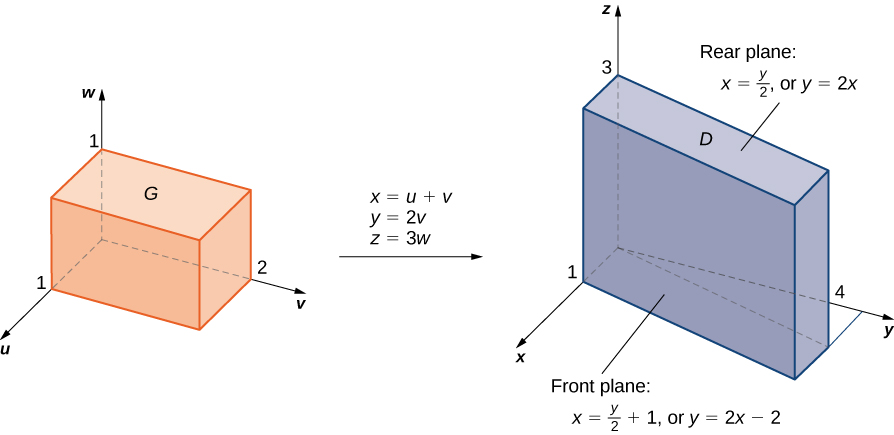
Now we can calculate the Jacobian for the transformation:
\[J(u,v,w)=|\begin{array}{lllll}\frac{∂x}{∂u} & & \frac{∂x}{∂v} & & \frac{∂x}{∂w} \\ \frac{∂y}{∂u} & & \frac{∂y}{∂v} & & \frac{∂y}{∂w} \\ \frac{∂z}{∂u} & & \frac{∂z}{∂v} & & \frac{∂z}{∂w}\end{array}|=|\begin{array}{lllll}1 & & 1 & & 0 \\ 0 & & 2 & & 0 \\ 0 & & 0 & & 3\end{array}|=6.\]
The function to be integrated becomes
\[f(x,y,z)=x+\frac{z}{3}=u+v+\frac{3w}{3}=u+v+w.\]
We are now ready to put everything together and complete the problem.
\[\begin{array}{l} \\ \\ \\ \\ \,\int_{0}^{3}\,\int_{0}^{4}\,\int_{y\text{/}2}^{(y\text{/}2)+1}(x+\frac{z}{3})dx\,dy\,dz \\ \\ =\int_{0}^{1}\,\int_{0}^{2}\,\int_{0}^{1}(u+v+w)|J(u,v,w)|du\,dv\,dw=\int_{0}^{1}\,\int_{0}^{2}\,\int_{0}^{1}(u+v+w)|6|du\,dv\,dw \\ =6\int_{0}^{1}\,\int_{0}^{2}\,\int_{0}^{1}(u+v+w)du\,dv\,dw=6{\int_{0}^{1}\,\int_{0}^{2}[\frac{{u}^{2}}{2}+vu+wu]}_{0}^{1}dv\,dw \\ =6\int_{0}^{1}\,\int_{0}^{2}(\frac{1}{2}+v+w)dv\,dw=6{\int_{0}^{1}[\frac{1}{2}v+\frac{{v}^{2}}{2}+wv]}_{0}^{2}dw \\ =6\int_{0}^{1}(3+2w)dw=6{[3w+{w}^{2}]}_{0}^{1}=24.\end{array}\]
Let \(D\) be the region in \(xyz\text{-space}\) defined by \(1\le x\le 2,0\le xy\le 2,\text{and}\,0\le z\le 1.\)
Evaluate \(\underset{D}{∭}({x}^{2}y+3xyz)dx\,dy\,dz\) by using the transformation \(u=x,v=xy,\) and \(w=3z.\)
\(\int_{0}^{3}\,\int_{0}^{2}\,\int_{1}^{2}(\frac{v}{3}+\frac{vw}{3u})du\,dv\,dw=2+\text{ln}\,8\)
Key Concepts
- A transformation \(T\) is a function that transforms a region \(G\) in one plane (space) into a region \(R\) in another plane (space) by a change of variables. (See Example 1 and Example 2.)
- A transformation \(T:G\to R\) defined as \(T(u,v)=(x,y)\) \((\text{or}\,T(u,v,w)=(x,y,z))\) is said to be a one-to-one transformation if no two points map to the same image point. (See Example 1.)
- If \(f\) is continuous on \(R,\) then \(\underset{R}{∬}f(x,y)dA=\underset{S}{∬}f(g(u,v),h(u,v))|\frac{∂(x,y)}{∂(u,v)}|du\,dv.\) (See Example 5, Example 6, and Example 7.)
- If \(F\) is continuous on \(R,\) then
\[\begin{array}{ll}\underset{R}{∭}F(x,y,z)dV & =\underset{G}{∭}F(g(u,v,w),h(u,v,w),k(u,v,w))|\frac{∂(x,y,z)}{∂(u,v,w)}|du\,dv\,dw \\ & =\underset{G}{∭}H(u,v,w)|J(u,v,w)|du\,dv\,dw.\end{array}\]
(See Example 8 and Example 9.)
Section Exercises
In the following exercises, the function \(T:S\to R,T(u,v)=(x,y)\) on the region \(S=\{(u,v)|0\le u\le 1,0\le v\le 1\}\) bounded by the unit square is given, where \(R⊂{ℝ}^{2}\) is the image of \(S\) under \(T.\)
- Justify that the function \(T\) is a \({C}^{1}\) transformation.
- Find the images of the vertices of the unit square \(S\) through the function \(T.\)
- Determine the image \(R\) of the unit square \(S\) and graph it.
\(x=2u,y=3v\)
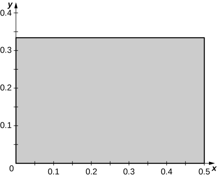
\(x=\frac{u}{2},y=\frac{v}{3}\)
a. \(T(u,v)=(g(u,v),h(u,v)),x=g(u,v)=\frac{u}{2}\) and \(y=h(u,v)=\frac{v}{3}.\) The functions \(g\) and \(h\) are continuous and differentiable, and the partial derivatives \({g}_{u}(u,v)=\frac{1}{2},\) \({g}_{v}(u,v)=0,{h}_{u}(u,v)=0\,\text{and}\,{h}_{v}(u,v)=\frac{1}{3}\) are continuous on \(S;\) b. \(T(0,0)=(0,0),\) \(T(1,0)=(\frac{1}{2},0),T(0,1)=(0,\frac{1}{3}),\) and \(T(1,1)=(\frac{1}{2},\frac{1}{3});\) c. \(R\) is the rectangle of vertices \((0,0),(\frac{1}{2},0),(\frac{1}{2},\frac{1}{3}),\text{and}\,(0,\frac{1}{3})\) in the \(xy\text{-plane;}\) the following figure.
\(x=u-v,y=u+v\)
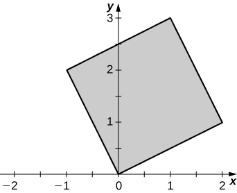
\(x=2u-v,y=u+2v\)
a. \(T(u,v)=(g(u,v),h(u,v)),x=g(u,v)=2u-v,\) and \(y=h(u,v)=u+2v.\) The functions \(g\) and \(h\) are continuous and differentiable, and the partial derivatives \({g}_{u}(u,v)=2,\) \({g}_{v}(u,v)=-1,\) \({h}_{u}(u,v)=1,\) and \({h}_{v}(u,v)=2\) are continuous on \(S;\) b. \(T(0,0)=(0,0),\) \(T(1,0)=(2,1),\) \(T(0,1)=(-1,2),\) and \(T(1,1)=(1,3);\) c. \(R\) is the sqaure of vertices \((0,0),(2,1),(1,3),\text{and}\,(-1,2)\) in the \(xy\text{-plane;}\) see the following figure.
\(x={u}^{2},y={v}^{2}\)
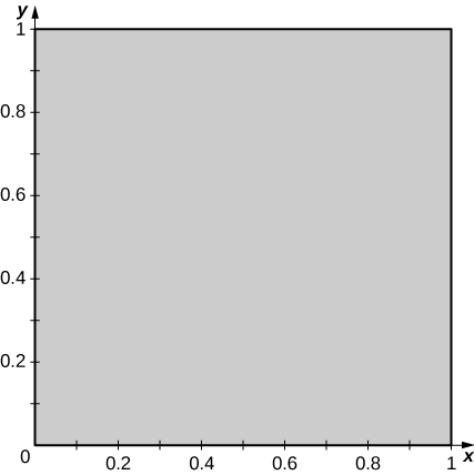
\(x={u}^{3},y={v}^{3}\)
a. \(T(u,v)=(g(u,v),h(u,v)),x=g(u,v)={u}^{3},\) and \(y=h(u,v)={v}^{3}.\) The functions \(g\) and \(h\) are continuous and differentiable, and the partial derivatives \({g}_{u}(u,v)=3{u}^{2},\) \({g}_{v}(u,v)=0,\) \({h}_{u}(u,v)=0,\) and \({h}_{v}(u,v)=3{v}^{2}\) are continuous on \(S;\) b. \(T(0,0)=(0,0),\) \(T(1,0)=(1,0),\) \(T(0,1)=(0,1),\) and \(T(1,1)=(1,1);\) c. \(R\) is the unit square in the \(xy\text{-plane;}\) see the following figure.
In the following exercises, determine whether the transformations \(T:S\to R\) are one-to-one or not.
\(x={u}^{2},y={v}^{2},\text{where}\,S\) is the rectangle of vertices \((-1,0),(1,0),(1,1),\text{and}\,(-1,1).\)
\(x={u}^{4},y={u}^{2}+v,\text{where}\,S\) is the triangle of vertices \((-2,0),(2,0),\text{and}\,(0,2).\)
\(T\) is not one-to-one: two points of \(S\) have the same image. Indeed, \(T(-2,0)=T(2,0)=(16,4).\)
\(x=2u,y=3v,\text{where}\,S\) is the square of vertices \((-1,1),(-1,-1),(1,-1),\text{and}\,(1,1).\)
\(T(u,v)=(2u-v,u),\) where \(S\) is the triangle of vertices \((-1,1),(-1,-1),\text{and}\,(1,-1).\)
\(T\) is one-to-one: We argue by contradiction. \(T({u}_{1},{v}_{1})=T({u}_{2},{v}_{2})\) implies \(2{u}_{1}-{v}_{1}=2{u}_{2}-{v}_{2}\) and \({u}_{1}={u}_{2}.\) Thus, \({u}_{1}={u}_{2}\) and \({v}_{1}={v}_{2}.\)
\(x=u+v+w,y=u+v,z=w,\) where \(S=R={ℝ}^{3}.\)
\(x={u}^{2}+v+w,y={u}^{2}+v,z=w,\) where \(S=R={ℝ}^{3}.\)
\(T\) is not one-to-one: \(T(1,v,w)=(-1,v,w)\)
In the following exercises, the transformations \(T:S\to R\) are one-to-one. Find their related inverse transformations \({T}^{-1}:R\to S.\)
\(x=4u,y=5v,\) where \(S=R={ℝ}^{2}.\)
\(x=u+2v,y=\text{-}u+v,\) where \(S=R={ℝ}^{2}.\)
\(u=\frac{x-2y}{3},v=\frac{x+y}{3}\)
\(x={e}^{2u+v},y={e}^{u-v},\) where \(S={ℝ}^{2}\) and \(R=\{(x,y)|x>0,y>0\}\)
\(x=\text{ln}\,u,y=\text{ln}(uv),\) where \(S=\{(u,v)|u>0,v>0\}\) and \(R={ℝ}^{2}.\)
\(u={e}^{x},v={e}^{\text{-}x+y}\)
\(x=u+v+w,y=3v,z=2w,\) where \(S=R={ℝ}^{3}.\)
\(x=u+v,y=v+w,z=u+w,\) where \(S=R={ℝ}^{3}.\)
\(u=\frac{x-y+z}{2},v=\frac{x+y-z}{2},w=\frac{\text{-}x+y+z}{2}\)
In the following exercises, the transformation \(T:S\to R,T(u,v)=(x,y)\) and the region \(R⊂{ℝ}^{2}\) are given. Find the region \(S⊂{ℝ}^{2}.\)
\(x=au,y=bv,R=\{(x,y)|{x}^{2}+{y}^{2}\le {a}^{2}{b}^{2}\},\) where \(a,b>0\)
\(x=au,y=bv,R=\{(x,y)|\frac{{x}^{2}}{{a}^{2}}+\frac{{y}^{2}}{{b}^{2}}\le 1\},\) where \(a,b>0\)
\(S=\{(u,v)|{u}^{2}+{v}^{2}\le 1\}\)
\(x=\frac{u}{a},y=\frac{v}{b},z=\frac{w}{c},\) \(R=\{(x,y)|{x}^{2}+{y}^{2}+{z}^{2}\le 1\},\) where \(a,b,c>0\)
\(x=au,y=bv,z=cw,R=\{(x,y)|\frac{{x}^{2}}{{a}^{2}}-\frac{{y}^{2}}{{b}^{2}}-\frac{{z}^{2}}{{c}^{2}}\le 1,z>0\},\) where \(a,b,c>0\)
\(R=\{(u,v,w)|{u}^{2}-{v}^{2}-{w}^{2}\le 1,w>0\}\)
In the following exercises, find the Jacobian \(J\) of the transformation.
\(x=u+2v,y=\text{-}u+v\)
\(x=\frac{{u}^{3}}{2},y=\frac{v}{{u}^{2}}\)
\(\frac{3}{2}\)
\(x={e}^{2u-v},y={e}^{u+v}\)
\(x=u{e}^{v},y={e}^{\text{-}v}\)
\(-1\)
\(x=u\,\text{cos}({e}^{v}),y=u\,\text{sin}({e}^{v})\)
\(x=v\,\text{sin}({u}^{2}),y=v\,\text{cos}({u}^{2})\)
\(2uv\)
\(x=u\,\text{cosh}\,v,y=u\,\text{sinh}\,v,z=w\)
\(x=v\,\text{cosh}(\frac{1}{u}),y=v\,\text{sinh}(\frac{1}{u}),z=u+{w}^{2}\)
\(\frac{2vw}{{u}^{2}}\text{or}\frac{2w\left(u+{w}^{2}\right)}{{u}^{2}}\)
\(x=u+v,y=v+w,z=u\)
\(x=u-v,y=u+v,z=u+v+w\)
\(2\)
The triangular region \(R\) with the vertices \((0,0),(1,1),\text{and}\,(1,2)\) is shown in the following figure.
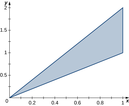
- Find a transformation \(T:S\to R,\) \(T(u,v)=(x,y)=(au+bv,cu+dv),\) where \(a,b,c,\) and \(d\) are real numbers with \(ad-bc\ne 0\) such that \({T}^{-1}(0,0)=(0,0),{T}^{-1}(1,1)=(1,0),\) and \({T}^{-1}(1,2)=(0,1).\)
- Use the transformation \(T\) to find the area \(A(R)\) of the region \(R.\)
The triangular region \(R\) with the vertices \((0,0),(2,0),\text{and}\,(1,3)\) is shown in the following figure.
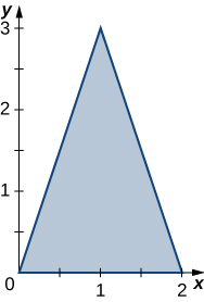
- Find a transformation \(T:S\to R,\) \(T(u,v)=(x,y)=(au+bv,cu+dv),\) where \(a,b,c\) and \(d\) are real numbers with \(ad-bc\ne 0\) such that \({T}^{-1}(0,0)=(0,0),\) \({T}^{-1}(2,0)=(1,0),\) and \({T}^{-1}(1,3)=(0,1).\)
- Use the transformation \(T\) to find the area \(A(R)\) of the region \(R.\)
a. \(T(u,v)=(2u+v,3v);\) b. The area of \(R\) is
\(A(R)=\int_{0}^{3}\,\int_{y\text{/}3}^{(6-y)\text{/}3}dx\,dy=\int_{0}^{1}\,\int_{0}^{1-u}|\frac{∂(x,y)}{∂(u,v)}|dv\,du=\int_{0}^{1}\,\int_{0}^{1-u}6dv\,du=3.\)
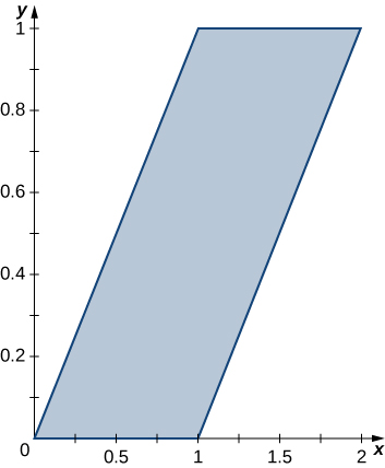
In the following exercises, use the transformation \(u=y-x,v=y,\) to evaluate the integrals on the parallelogram \(R\) of vertices \((0,0),(1,0),(2,1),\text{and}\,(1,1)\) shown in the following figure.
\(\underset{R}{∬}(y-x)dA\)
\(\underset{R}{∬}({y}^{2}-xy)dA\)
\(-\frac{1}{4}\)
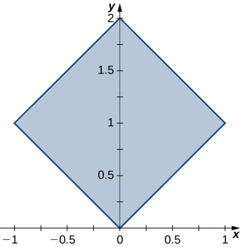
In the following exercises, use the transformation \(y-x=u,x+y=v\) to evaluate the integrals on the square \(R\) determined by the lines \(y=x,y=\text{-}x+2,y=x+2,\) and \(y=\text{-}x\) shown in the following figure.
\(\underset{R}{∬}{e}^{x+y}dA\)
\(\underset{R}{∬}\text{sin}(x-y)dA\)
\(-1+\text{cos}\,2\)
In the following exercises, use the transformation \(x=u,5y=v\) to evaluate the integrals on the region \(R\) bounded by the ellipse \({x}^{2}+25{y}^{2}=1\) shown in the following figure.
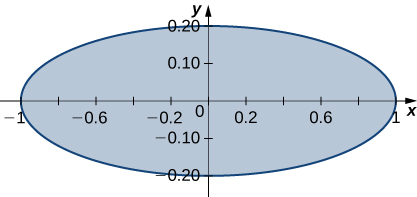
\(\underset{R}{∬}\sqrt{{x}^{2}+25{y}^{2}}\,dA\)
\({\underset{R}{∬}({x}^{2}+25{y}^{2})}^{2}dA\)
\(\frac{\pi }{15}\)
In the following exercises, use the transformation \(u=x+y,v=x-y\) to evaluate the integrals on the trapezoidal region \(R\) determined by the points \((1,0),(2,0),(0,2\text{)},\text{and}\,(0,1)\) shown in the following figure.
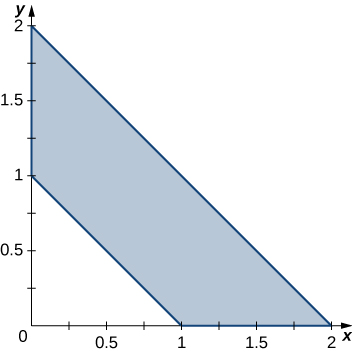
\(\underset{R}{∬}({x}^{2}-2xy+{y}^{2}){e}^{x+y}dA\)
\(\underset{R}{∬}({x}^{3}+3{x}^{2}y+3x{y}^{2}+{y}^{3})dA\)
\(\frac{31}{5}\)
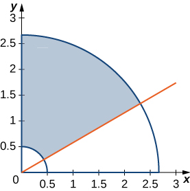
The circular annulus sector \(R\) bounded by the circles \(4{x}^{2}+4{y}^{2}=1\) and \(9{x}^{2}+9{y}^{2}=64,\) the line \(x=y\sqrt{3},\) and the \(y\text{-axis}\) is shown in the following figure. Find a transformation \(T\) from a rectangular region \(S\) in the \(rθ\text{-plane}\) to the region \(R\) in the \(xy\text{-plane.}\) Graph \(S.\)
The solid \(R\) bounded by the circular cylinder \({x}^{2}+{y}^{2}=9\) and the planes \(z=0,z=1,\) \(x=0,\text{and}\,y=0\) is shown in the following figure. Find a transformation \(T\) from a cylindrical box \(S\) in \(rθz\text{-space}\) to the solid \(R\) in \(xyz\text{-space}.\)
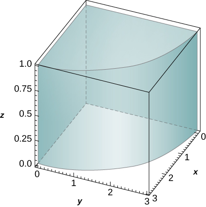
\(T(r,θ,z)=(r\,\text{cos}\,θ,r\,\text{sin}\,θ,z);S=[0,3]\,\times \,[0,\frac{\pi }{2}]\,\times \,[0,1]\) in the \(rθz\text{-space}\)
Show that \(\underset{R}{∬}f(\sqrt{\frac{{x}^{2}}{3}+\frac{{y}^{2}}{3}})dA=2\pi \sqrt{15}\int_{0}^{1}f(ρ)ρ\,dρ,\) where \(f\) is a continuous function on \([0,1]\) and \(R\) is the region bounded by the ellipse \(5{x}^{2}+3{y}^{2}=15.\)
Show that \(\underset{R}{∭}f(\sqrt{16{x}^{2}+4{y}^{2}+{z}^{2}})dV=\frac{\pi }{2}\int_{0}^{1}f(ρ){ρ}^{2}dρ,\) where \(f\) is a continuous function on \([0,1]\) and \(R\) is the region bounded by the ellipsoid \(16{x}^{2}+4{y}^{2}+{z}^{2}=1.\)
[T] Find the area of the region bounded by the curves \(xy=1,xy=3,y=2x,\) and \(y=3x\) by using the transformation \(u=xy\) and \(v=\frac{y}{x}.\) Use a computer algebra system (CAS) to graph the boundary curves of the region \(R.\)
[T] Find the area of the region bounded by the curves \(xy=2,xy=3,y=x,\) and \(y=2x\) by using the transformation \(u=xy\) and \(v=\frac{y}{x}.\)
The area of the region is \(\frac{ln2}{2}.\) A graph of the region is:
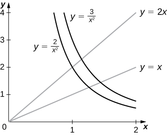
Evaluate the triple integral \(\int_{0}^{1}\,\int_{1}^{2}\,\int_{z}^{z+1}(y+1)dx\,dy\,dz\) by using the transformation \(u=x-z,\) \(v=3y,\text{and}\,w=\frac{z}{2}.\)
Evaluate the triple integral \(\int_{0}^{2}\,\int_{4}^{6}\,\int_{3z}^{3z+2}(5-4y)dx\,dz\,dy\) by using the transformation \(u=x-3z,v=4y,\text{and}\,w=z.\)
\(8\)
A transformation \(T:{ℝ}^{2}\to {ℝ}^{2},T(u,v)=(x,y)\) of the form \(x=au+bv,y=cu+dv,\) where \(a,b,c,\text{and}\,d\) are real numbers, is called linear. Show that a linear transformation for which \(ad-bc\ne 0\) maps parallelograms to parallelograms.
The transformation \({T}_{θ}:{ℝ}^{2}\to {ℝ}^{2},{T}_{θ}(u,v)=(x,y),\) where \(x=u\,\text{cos}\,θ-v\,\text{sin}\,θ,\) \(y=u\,\text{sin}\,θ+v\,\text{cos}\,θ,\) is called a rotation of angle \(θ.\) Show that the inverse transformation of \({T}_{θ}\) satisfies \({T}_{θ}{}^{-1}={T}_{\text{-}θ},\) where \({T}_{\text{-}θ}\) is the rotation of angle \(\text{-}θ.\)
[T] Use the results of the previous exercise to find the region \(S\) in the \(uv\text{-plane}\) whose image through a rotation of angle \(\frac{\pi }{4}\) is the region \(R\) enclosed by the ellipse \({x}^{2}+4{y}^{2}=1.\) Use a CAS to answer the following questions.
- Graph the region \(S.\)
- Evaluate the integral \(\underset{S}{∬}{e}^{-2uv}du\,dv.\) Round your answer to two decimal places.
[T] The transformations \({T}_{i}:{ℝ}^{2}\to {ℝ}^{2},\) \(i=1\text{,…,}\,4,\) defined by \({T}_{1}(u,v)=(u,\text{-}v),\) \({T}_{2}(u,v)=(\text{-}u,v),{T}_{3}(u,v)=(\text{-}u,\text{-}v),\) and \({T}_{4}(u,v)=(v,u)\) are called reflections about the \(x\text{-axis},y\text{-axis},\) origin, and the line \(y=x,\) respectively.
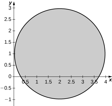
- Find the image of the region \(S=\{(u,v)|{u}^{2}+{v}^{2}-2u-4v+1\le 0\}\) in the \(xy\text{-plane}\) through the transformation \({T}_{1}∘{T}_{2}∘{T}_{3}∘{T}_{4}.\)
- Use a CAS to graph the image of \(S.\)
- Evaluate the integral \(\underset{S}{∬}\text{sin}({u}^{2})du\,dv\) by using a CAS. Round your answer to two decimal places.
a. \(R=\{(x,y)|{y}^{2}+{x}^{2}-2y-4x+1\le 0\};\) b. \(R\) is graphed in the following figure;
c. \(3.16\)
[T] The transformation \({T}_{k,1,1}:{ℝ}^{3}\to {ℝ}^{3},{T}_{k,1,1}(u,v,w)=(x,y,z)\) of the form \(x=ku,\) \(y=v,z=w,\) where \(k\ne 1\) is a positive real number, is called a stretch if \(k>1\) and a compression if \(0<k<1\) in the \(x\text{-direction}\text{.}\) Use a CAS to evaluate the integral \(\underset{S}{∭}{e}^{\text{-}(4{x}^{2}+9{y}^{2}+25{z}^{2})}dx\,dy\,dz\) on the solid \(S=\{(x,y,z)|4{x}^{2}+9{y}^{2}+25{z}^{2}\le 1\}\) by considering the compression \({T}_{2,3,5}(u,v,w)=(x,y,z)\) defined by \(x=\frac{u}{2},y=\frac{v}{3},\) and \(z=\frac{w}{5}.\) Round your answer to four decimal places.
[T] The transformation \({T}_{a,0}:{ℝ}^{2}\to {ℝ}^{2},{T}_{a,0}(u,v)=(u+av,v),\) where \(a\ne 0\) is a real number, is called a shear in the \(x\text{-direction}\text{.}\) The transformation, \({T}_{0,b}:{ℝ}^{2}\to {ℝ}^{2},{T}_{0,b}(u,v)=(u,bu+v),\) where \(b\ne 0\) is a real number, is called a shear in the \(y\text{-direction}\text{.}\)
- Find transformations \({T}_{0,2}∘{T}_{3,0}.\)
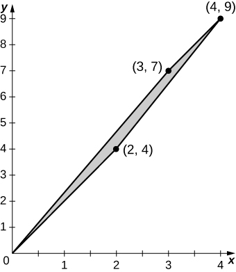
- Find the image \(R\) of the trapezoidal region \(S\) bounded by \(u=0,v=0,v=1,\) and \(v=2-u\) through the transformation \({T}_{0,2}∘{T}_{3,0}.\)
- Use a CAS to graph the image \(R\) in the \(xy\text{-plane}\text{.}\)
- Find the area of the region \(R\) by using the area of region \(S.\)
a. \({T}_{0,2}∘{T}_{3,0}(u,v)=(u+3v,2u+7v);\) b. The image \(R\) is the quadrilateral of vertices \((0,0),(3,7),(2,4),\text{and}\,(4,9);\) c. \(S\) is graphed in the following figure;
d. \(\frac{3}{2}\)
Use the transformation, \(x=au,y=av,z=cw\) and spherical coordinates to show that the volume of a region bounded by the spheroid \(\frac{{x}^{2}+{y}^{2}}{{a}^{2}}+\frac{{z}^{2}}{{c}^{2}}=1\) is \(\frac{4\pi {a}^{2}c}{3}.\)
Find the volume of a football whose shape is a spheroid \(\frac{{x}^{2}+{y}^{2}}{{a}^{2}}+\frac{{z}^{2}}{{c}^{2}}=1\) whose length from tip to tip is \(11\) inches and circumference at the center is \(22\) inches. Round your answer to two decimal places.
\(\frac{2662}{3\pi }≃282.45{\,\text{in}}^{3}\)
[T] Lamé ovals (or superellipses) are plane curves of equations \({(\frac{x}{a})}^{n}+{(\frac{y}{b})}^{n}=1,\) where a, b, and n are positive real numbers.
- Use a CAS to graph the regions \(R\) bounded by Lamé ovals for \(a=1,b=2,n=4\) and \(n=6,\) respectively.
- Find the transformations that map the region \(R\) bounded by the Lamé oval \({x}^{4}+{y}^{4}=1,\) also called a squircle and graphed in the following figure, into the unit disk.
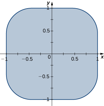
- Use a CAS to find an approximation of the area \(A(R)\) of the region \(R\) bounded by \({x}^{4}+{y}^{4}=1.\) Round your answer to two decimal places.
[T] Lamé ovals have been consistently used by designers and architects. For instance, Gerald Robinson, a Canadian architect, has designed a parking garage in a shopping center in Peterborough, Ontario, in the shape of a superellipse of the equation \({(\frac{x}{a})}^{n}+{(\frac{y}{b})}^{n}=1\) with \(\frac{a}{b}=\frac{9}{7}\) and \(n=e.\) Use a CAS to find an approximation of the area of the parking garage in the case \(a=900\) yards, \(b=700\) yards, and \(n=2.72\) .
\(A(R)=2,177,216 {\text{yd}}^{2}\)
Chapter Review Exercises
True or False? Justify your answer with a proof or a counterexample.
\(\int_{a}^{b}\,\int_{c}^{d}f(x,y)dy\,dx=\int_{c}^{d}\,\int_{a}^{b}f(x,y)dy\,dx\)
Fubini’s theorem can be extended to three dimensions, as long as \(f\) is continuous in all variables.
True.
The integral \(\int_{0}^{2\pi }\,\int_{0}^{1}\,\int_{r}^{1}dz\,dr\,dθ\) represents the volume of a right cone.
The Jacobian of the transformation \(x={u}^{2}-2v,y=3v-2uv\) is given by \(-4{u}^{2}+6u+4v.\)
False.
Evaluate the following integrals.
\(\underset{R}{∬}(5{x}^{3}{y}^{2}-{y}^{2})dA,R=\{(x,y)|0\le x\le 2,1\le y\le 4\}\)
\(\underset{D}{∬}\frac{y}{3{x}^{2}+1}dA,D=\{(x,y)|0\le x\le 1,\text{-}x\le y\le x\}\)
0
\(\underset{D}{∬}\text{sin}({x}^{2}+{y}^{2})dA\) where \(D\) is a disk of radius \(2\) centered at the origin
\(\int_{0}^{1}\,\int_{y}^{1}xy{e}^{{x}^{2}}dx\,dy\)
\(\frac{1}{4}\)
\(\int_{-1}^{1}\,\int_{0}^{z}\,\int_{0}^{x-z}6dy\,dx\,dz\)
\(\underset{R}{∭}3y\,dV,\) where \(R=\{(x,y,z)|0\le x\le 1,0\le y\le x,0\le z\le \sqrt{9-{y}^{2}}\}\)
1.475
\(\int_{0}^{2}\,\int_{0}^{2\pi }\,\int_{r}^{1}r\,dz\,dθ\,dr\)
\(\int_{0}^{2\pi }\,\int_{0}^{\pi \text{/}2}\,\int_{1}^{3}{ρ}^{2}\text{sin}(φ)dρ\,dφ\,dθ\)
\(\frac{52}{3}\pi\)
\(\int_{0}^{1}\,\int_{\text{-}\sqrt{1-{x}^{2}}}^{\sqrt{1-{x}^{2}}}\,\int_{\text{-}\sqrt{1-{x}^{2}-{y}^{2}}}^{\sqrt{1-{x}^{2}-{y}^{2}}}dz\,dy\,dx\)
For the following problems, find the specified area or volume.
The area of region enclosed by one petal of \(r=\text{cos}(4θ).\)
\(\frac{\pi }{16}\)
The volume of the solid that lies between the paraboloid \(z=2{x}^{2}+2{y}^{2}\) and the plane \(z=8.\)
The volume of the solid bounded by the cylinder \({x}^{2}+{y}^{2}=16\) and from \(z=1\) and \(z+x=2.\)
\(16\pi \approx 50.265\)
The volume of the intersection between two spheres of radius 1, the top whose center is \((0,0,0.25)\) and the bottom, which is centered at \((0,0,0).\)
For the following problems, find the center of mass of the region.
\(ρ(x,y)=xy\) on the circle with radius \(1\) in the first quadrant only.
\((\frac{8}{15},\frac{8}{15})\)
\(ρ(x,y)=(y+1)\sqrt{x}\) in the region bounded by \(y={e}^{x},\) \(y=0,\) and \(x=1.\)
\(ρ(x,y,z)=z\) on the inverted cone with radius \(2\) and height \(2.\)
\((0,0,\frac{4}{5})\)
The volume an ice cream cone that is given by the solid above \(z=\sqrt{({x}^{2}+{y}^{2})}\) and below \({z}^{2}+{x}^{2}+{y}^{2}=z.\)
The following problems examine Mount Holly in the state of Michigan. Mount Holly is a landfill that was converted into a ski resort. The shape of Mount Holly can be approximated by a right circular cone of height \(1100\) ft and radius \(6000\) ft.
If the compacted trash used to build Mount Holly on average has a density \(400{\,\text{lb/ft}}^{3},\) find the amount of work required to build the mountain.
\(1.452\pi \,\times \,{10}^{15}\) ft-lb
In reality, it is very likely that the trash at the bottom of Mount Holly has become more compacted with all the weight of the above trash. Consider a density function with respect to height: the density at the top of the mountain is still density \(400{\,\text{lb/ft}}^{3}\) and the density increases. Every \(100\) feet deeper, the density doubles. What is the total weight of Mount Holly?
The following problems consider the temperature and density of Earth’s layers.
[T] The temperature of Earth’s layers is exhibited in the table below. Use your calculator to fit a polynomial of degree \(3\) to the temperature along the radius of the Earth. Then find the average temperature of Earth. (Hint: begin at \(0\) in the inner core and increase outward toward the surface)
| Layer | Depth from center (km) | Temperature \(\text{°}C\) |
| Rocky Crust | 0 to 40 | 0 |
| Upper Mantle | 40 to 150 | 870 |
| Mantle | 400 to 650 | 870 |
| Inner Mantel | 650 to 2700 | 870 |
| Molten Outer Core | 2890 to 5150 | 4300 |
| Inner Core | 5150 to 6378 | 7200 |
\(y=-1.238\,\times \,{10}^{-7}{x}^{3}+0.001196{x}^{2}-3.666x+7208;\) average temperature approximately \({2800}^{\text{°}}C\)
[T] The density of Earth’s layers is displayed in the table below. Using your calculator or a computer program, find the best-fit quadratic equation to the density. Using this equation, find the total mass of Earth.
| Layer | Depth from center (km) | Density (g/cm3) |
| Inner Core | \(0\) | \(12.95\) |
| Outer Core | \(1228\) | \(11.05\) |
| Mantle | \(3488\) | \(5.00\) |
| Upper Mantle | \(6338\) | \(3.90\) |
| Crust | \(6378\) | \(2.55\) |
The following problems concern the Theorem of Pappus (see Moments and Centers of Mass for a refresher), a method for calculating volume using centroids. Assuming a region \(R,\) when you revolve around the \(x\text{-axis}\) the volume is given by \({V}_{x}=2\pi A\bar{\left(y\right)},\) and when you revolve around the \(\text{y-axis}\) the volume is given by \({V}_{y}=2\pi A\left(\bar{x}\right),\) where \(A\) is the area of \(R.\) Consider the region bounded by \({x}^{2}+{y}^{2}=1\) and above \(y=x+1.\)
Find the volume when you revolve the region around the \(x\text{-axis.}\)
\(\frac{\pi }{3}\)
Find the volume when you revolve the region around the \(y\text{-axis.}\)
Glossary
- Jacobian
- the Jacobian \(J(u,v)\) in two variables is a \(2\,\times \,2\) determinant:
the Jacobian \(J(u,v,w)\) in three variables is a \(3\,\times \,3\) determinant: - one-to-one transformation
- a transformation \(T:G\to R\) defined as \(T(u,v)=(x,y)\) is said to be one-to-one if no two points map to the same image point
- planar transformation
- a function \(T\) that transforms a region \(G\) in one plane into a region \(R\) in another plane by a change of variables
- transformation
- a function that transforms a region \(G\) in one plane into a region \(R\) in another plane by a change of variables