Section 5.2Double Integrals over General Regions
In Double Integrals over Rectangular Regions, we studied the concept of double integrals and examined the tools needed to compute them. We learned techniques and properties to integrate functions of two variables over rectangular regions. We also discussed several applications, such as finding the volume bounded above by a function over a rectangular region, finding area by integration, and calculating the average value of a function of two variables.
In this section we consider double integrals of functions defined over a general bounded region \(D\) on the plane. Most of the previous results hold in this situation as well, but some techniques need to be extended to cover this more general case.
General Regions of Integration
An example of a general bounded region \(D\) on a plane is shown in Figure 1. Since \(D\) is bounded on the plane, there must exist a rectangular region \(R\) on the same plane that encloses the region \(D,\) that is, a rectangular region \(R\) exists such that \(D\) is a subset of \(R(D⊆R).\)
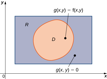
Suppose \(z=f(x,y)\) is defined on a general planar bounded region \(D\) as in Figure 1. In order to develop double integrals of \(f\) over \(D,\) we extend the definition of the function to include all points on the rectangular region \(R\) and then use the concepts and tools from the preceding section. But how do we extend the definition of \(f\) to include all the points on \(R?\) We do this by defining a new function \(g(x,y)\) on \(R\) as follows:
\[g(x,y)=\left\{\begin{array}{ll}f(x,y) & \text{if}\,(x,y)\,\text{is in}\,D \\ 0 & \text{if}\,(x,y)\,\text{is in}\,R\,\text{but not in}\,D\end{array}\right.\]
Note that we might have some technical difficulties if the boundary of \(D\) is complicated. So we assume the boundary to be a piecewise smooth and continuous simple closed curve. Also, since all the results developed in Double Integrals over Rectangular Regions used an integrable function \(f(x,y),\) we must be careful about \(g(x,y)\) and verify that \(g(x,y)\) is an integrable function over the rectangular region \(R.\) This happens as long as the region \(D\) is bounded by simple closed curves. For now we will concentrate on the descriptions of the regions rather than the function and extend our theory appropriately for integration.
We consider two types of planar bounded regions.
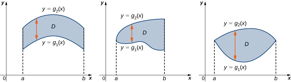
A region \(D\) in the \((x,y)\) -plane is of Type I if it lies between two vertical lines and the graphs of two continuous functions \({g}_{1}(x)\) and \({g}_{2}(x).\) That is (Figure 2),
\[D=\{(x,y)|a\le x\le b,{g}_{1}(x)\le y\le {g}_{2}(x)\}.\]
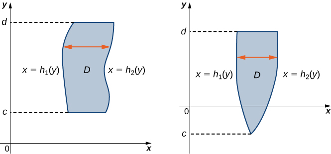
A region \(D\) in the \(xy\) plane is of Type II if it lies between two horizontal lines and the graphs of two continuous functions \({h}_{1}(y)\,\text{and}\,{h}_{2}(y).\) That is (Figure 3),
\[D=\{(x,y)|c\le y\le d,{h}_{1}(y)\le x\le {h}_{2}(y)\}.\]
Consider the region in the first quadrant between the functions \(y=\sqrt{x}\) and \(y={x}^{3}\) (Figure 4). Describe the region first as Type I and then as Type II.
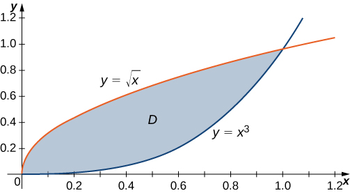
Sketch the region and determine which curve bounds it above and below for Type I, then which bounds it left and right for Type II.
When describing a region as Type I, we need to identify the function that lies above the region and the function that lies below the region. Here, region \(D\) is bounded above by \(y=\sqrt{x}\) and below by \(y={x}^{3}\) in the interval for \(x\,\text{in}\,[0,1].\) Hence, as Type I, \(D\) is described as the set \(\{(x,y)|0\le x\le 1,{x}^{3}\le y\le \sqrt{x}\}.\)
However, when describing a region as Type II, we need to identify the function that lies on the left of the region and the function that lies on the right of the region. Here, the region \(D\) is bounded on the left by \(x={y}^{2}\) and on the right by \(x=\sqrt[3]{y}\) in the interval for y in \([0,1].\) Hence, as Type II, \(D\) is described as the set \(\{(x,y)|0\le y\le 1,{y}^{2}\le x\le \sqrt[3]{y}\}.\)
Consider the region in the first quadrant between the functions \(y=2x\) and \(y={x}^{2}.\) Describe the region first as Type I and then as Type II.
Type I and Type II are expressed as \(\{(x,y)|0\le x\le 2,{x}^{2}\le y\le 2x\}\) and \(\{(x,y)|0\le y\le 4,\frac{1}{2}y\le x\le \sqrt{y}\},\) respectively.
Double Integrals over Nonrectangular Regions
To develop the concept and tools for evaluation of a double integral over a general, nonrectangular region, we need to first understand the region and be able to express it as Type I or Type II or a combination of both. Without understanding the regions, we will not be able to decide the limits of integrations in double integrals. As a first step, let us look at the following theorem.
Suppose \(g(x,y)\) is the extension to the rectangle \(R\) of the integrable function \(f(x,y)\) defined on the region \(D\) , where \(D\) is inside \(R\) . Sample regions are as shown in Figure 1. Then \(g(x,y)\) is integrable and we define the double integral of \(f(x,y)\) over \(D\) by
\[\underset{D}{∬}f(x,y)dA=\underset{R}{∬}g(x,y)dA.\]
The right-hand side of this equation is what we have seen before, so this theorem is reasonable because \(R\) is a rectangle and \(\underset{R}{∬}g(x,y)dA\) has been discussed in the preceding section. Also, the equality works because the values of \(g(x,y)\) are \(0\) for any point \((x,y)\) that lies outside \(D,\) and hence these points do not add anything to the integral. However, it is important that the rectangle \(R\) contains the region \(D.\)
As a matter of fact, if the region \(D\) is bounded by smooth curves on a plane and we are able to describe it as Type I or Type II or a mix of both, then we can use the following theorem and not have to find a rectangle \(R\) containing the region.
For a function \(f(x,y)\) that is continuous on a region \(D\) of Type I, we have
\[\underset{D}{∬}f(x,y)dA=\underset{D}{∬}f(x,y)dy\,dx=\int_{a}^{b}[\int_{{g}_{1}(x)}^{{g}_{2}(x)}f(x,y)dy]dx.\]
Similarly, for a function \(f(x,y)\) that is continuous on a region \(D\) of Type II, we have
\[\underset{D}{∬}f(x,y)dA=\underset{D}{∬}f(x,y)dx\,dy=\int_{c}^{d}[\int_{{h}_{1}(y)}^{{h}_{2}(y)}f(x,y)dx]dy.\]
The integral in each of these expressions is an iterated integral, similar to those we have seen before. Notice that, in the inner integral in the first expression, we integrate \(f(x,y)\) with \(x\) being held constant and the limits of integration being \({g}_{1}(x)\,\text{and}\,{g}_{2}(x).\) In the inner integral in the second expression, we integrate \(f(x,y)\) with \(y\) being held constant and the limits of integration are \({h}_{1}(y)\,\text{and}\,{h}_{2}(y).\)
Evaluate the integral \(\underset{D}{∬}{x}^{2}{e}^{xy}dA\) where \(D\) is shown in Figure 5.
Set up D as a Type I region first, writing the inequalities for x and y, then convert to an iterated integral.
First construct the region \(D\) as a Type I region (Figure 5). Here \(D=\{(x,y)|0\le x\le 2,\frac{1}{2}x\le y\le 1\}.\) Then we have
\[\underset{D}{∬}{x}^{2}{e}^{xy}dA=\int_{x=0}^{x=2}\,\int_{y=1\text{/}2x}^{y=1}{x}^{2}{e}^{xy}dy\,dx.\]
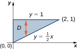
Therefore, we have
\[\begin{array}{lllll}\int_{x=0}^{x=2}\,\int_{y=\frac{1}{2}x}^{y=1}{x}^{2}{e}^{xy}dy\,dx & =\int_{x=0}^{x=2}[\int_{y=1\text{/}2x}^{y=1}{x}^{2}{e}^{xy}dy]dx & & & \text{Iterated integral for a Type I region.} \\ & =\int_{x=0}^{x=2}{[{x}^{2}\frac{{e}^{xy}}{x}]|}_{y=1\text{/}2x}^{y=1}dx & & & \begin{array}{l}\text{Integrate with respect to}\,y\,\text{using} \\ u\text{-substitution with}\,u=xy\,\text{where}\,x\,\text{is held} \\ \text{constant.}\end{array} \\ & =\int_{x=0}^{x=2}[x{e}^{x}-x{e}^{{x}^{2}\text{/}2}]dx & & & \begin{array}{l}\text{Integrate with respect to}\,x\,\text{using} \\ u\text{-substitution with}\,u=\frac{1}{2}{x}^{2}.\end{array} \\ & ={[x{e}^{x}-{e}^{x}-{e}^{\frac{1}{2}{x}^{2}}]|}_{x=0}^{x=2}=2 & & & \end{array}\]
In Example 2, we could have looked at the region in another way, such as \(D=\{(x,y)|0\le y\le 1,0\le x\le 2y\}\) (Figure 6).
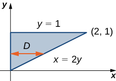
This is a Type II region and the integral would then look like
\[\underset{D}{∬}{x}^{2}{e}^{xy}dA=\int_{y=0}^{y=1}\,\int_{x=0}^{x=2y}{x}^{2}{e}^{xy}dx\,dy.\]
However, if we integrate first with respect to \(x,\) this integral is lengthy to compute because we have to use integration by parts twice.
Evaluate the integral \(\underset{D}{∬}(3{x}^{2}+{y}^{2})dA\) where \(=\{(x,y)|-2\le y\le 3,{y}^{2}-3\le x\le y+3\}.\)
Compare describing D as Type I versus Type II and choose the simpler Type II description before setting up the iterated integral.
Notice that \(D\) can be seen as either a Type I or a Type II region, as shown in Figure 7. However, in this case describing \(D\) as Type \(\text{I}\) is more complicated than describing it as Type II. Therefore, we use \(D\) as a Type II region for the integration.
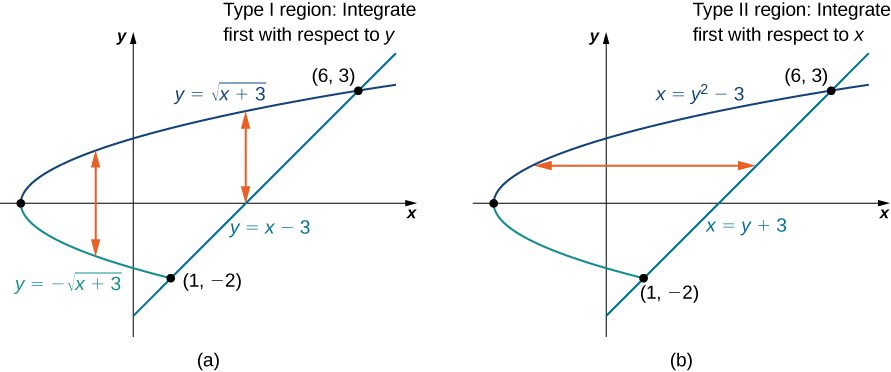
Choosing this order of integration, we have
\[\begin{array}{lllll}\underset{D}{∬}(3{x}^{2}+{y}^{2})dA & =\int_{y=-2}^{y=3}\,\int_{x={y}^{2}-3}^{x=y+3}(3{x}^{2}+{y}^{2})dx\,dy & & & \text{Iterated integral, Type II region.} \\ & ={\int_{y=-2}^{y=3}({x}^{3}+x{y}^{2})|}_{{y}^{2}-3}^{y+3}dy & & & \text{Integrate with respect to}\,x. \\ & =\int_{y=-2}^{y=3}({(y+3)}^{3}+(y+3){y}^{2}-{({y}^{2}-3)}^{3}-({y}^{2}-3){y}^{2})dy & & & \\ & =\int_{-2}^{3}(54+27y-12{y}^{2}+2{y}^{3}+8{y}^{4}-{y}^{6})dy & & & \text{Integrate with respect to}\,y. \\ & ={[54y+\frac{27{y}^{2}}{2}-4{y}^{3}+\frac{{y}^{4}}{2}+\frac{8{y}^{5}}{5}-\frac{{y}^{7}}{7}]|}_{-2}^{3} & & & \\ & =\frac{2375}{7}. & & & \end{array}\]
Sketch the region \(D\) and evaluate the iterated integral \(\underset{D}{∬}xy\,dy\,dx\) where \(D\) is the region bounded by the curves \(y=\text{cos}\,x\) and \(y=\text{sin}\,x\) in the interval \([-3\pi \text{/}4,\pi \text{/}4].\)
\(\pi \text{/}4\)
Recall from Double Integrals over Rectangular Regions the properties of double integrals. As we have seen from the examples here, all these properties are also valid for a function defined on a nonrectangular bounded region on a plane. In particular, property \(3\) states:
If \(R=S∪T\) and \(S∩T=\varnothing\) except at their boundaries, then
\[\underset{R}{∬}f(x,y)dA=\underset{S}{∬}f(x,y)dA+\underset{T}{∬}f(x,y)dA.\]
Similarly, we have the following property of double integrals over a nonrectangular bounded region on a plane.
Suppose the region \(D\) can be expressed as \(D={D}_{1}∪{D}_{2}\) where \({D}_{1}\) and \({D}_{2}\) do not overlap except at their boundaries. Then
\[\underset{D}{∬}f(x,y)dA=\underset{{D}_{1}}{∬}f(x,y)dA+\underset{{D}_{2}}{∬}f(x,y)dA.\]
This theorem is particularly useful for nonrectangular regions because it allows us to split a region into a union of regions of Type I and Type II. Then we can compute the double integral on each piece in a convenient way, as in the next example.
Express the region \(D\) shown in Figure 8 as a union of regions of Type I or Type II, and evaluate the integral
\[\underset{D}{∬}(2x+5y)dA.\]
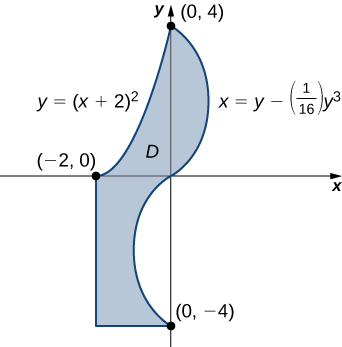
Break the region into pieces D1, D2, D3 that are each individually Type I or Type II, then sum the integrals over each piece.
The region \(D\) is not easy to decompose into any one type; it is actually a combination of different types. So we can write it as a union of three regions \({D}_{1},{D}_{2},\text{and}\,{D}_{3}\) where, \({D}_{1}=\{(x,y)|-2\le x\le 0,0\le y\le {(x+2)}^{2}\},\) \({D}_{2}=\{(x,y)|0\le y\le 4,0\le x\le (y-\frac{1}{16}{y}^{3})\},\) \({D}_{3}=\left(\left(x,y\right)-4\le y\le 0,-2\le x\le y-\frac{{y}^{3}}{16}\right).\) These regions are illustrated more clearly in Figure 9.
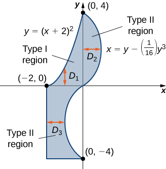
Here \({D}_{1}\) is Type \(\text{I}\) and \({D}_{2}\) and \({D}_{3}\) are both of Type II. Hence,
\[\begin{array}{ll}\underset{D}{∬}(2x+5y)dA & =\underset{{D}_{1}}{∬}(2x+5y)dA+\underset{{D}_{2}}{∬}(2x+5y)dA+\underset{{D}_{3}}{∬}(2x+5y)dA \\ & =\int_{x=-2}^{x=0}\,\int_{y=0}^{y={(x+2)}^{2}}(2x+5y)dy\,dx+\int_{y=0}^{y=4}\,\int_{x=0}^{x=y-(1\text{/}16){y}^{3}}(2+5y)dx\,dy+\int_{y=-4}^{y=0}\,\int_{x=-2}^{x=y-(1\text{/}16){y}^{3}}(2x+5y)dx\,dy \\ & =\int_{x=-2}^{x=0}[\frac{1}{2}{(2+x)}^{2}(20+24x+5{x}^{2})]dx+\int_{y=0}^{y=4}[\frac{1}{256}{y}^{6}-\frac{7}{16}{y}^{4}+6{y}^{2}]dy \\ & \,+\int_{y=-4}^{y=0}[\frac{1}{256}{y}^{6}-\frac{7}{16}{y}^{4}+6{y}^{2}+10y-4]dy \\ & =\frac{40}{3}+\frac{1664}{35}-\frac{1696}{35}=\frac{1304}{105}.\end{array}\]
Now we could redo this example using a union of two Type II regions (see the Checkpoint).
Consider the region bounded by the curves \(y=\text{ln}\,x\) and \(y={e}^{x}\) in the interval \([1,2].\) Decompose the region into smaller regions of Type II.
\(\{(x,y)|0\le y\le ln2,1\le x\le {e}^{y}\}∪\{(x,y)|ln2\le y\le e,1\le x\le 2\}∪\{(x,y)|e\le y\le {e}^{2},\text{ln}\,y\le x\le 2\}\)
Redo Example 4 using a union of two Type II regions.
Same as in the example shown.
Changing the Order of Integration
As we have already seen when we evaluate an iterated integral, sometimes one order of integration leads to a computation that is significantly simpler than the other order of integration. Sometimes the order of integration does not matter, but it is important to learn to recognize when a change in order will simplify our work.
Reverse the order of integration in the iterated integral \(\int_{x=0}^{x=\sqrt{2}}\,\int_{y=0}^{y=2-{x}^{2}}x{e}^{{x}^{2}}dy\,dx.\) Then evaluate the new iterated integral.
Rewrite the Type I region as Type II by solving y=2-x² for x, then swap the order of integration.
The region as presented is of Type I. To reverse the order of integration, we must first express the region as Type II. Refer to Figure 10.
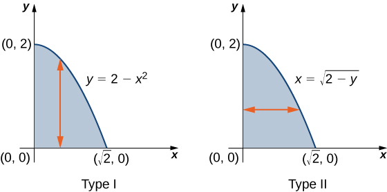
We can see from the limits of integration that the region is bounded above by \(y=2-{x}^{2}\) and below by \(y=0,\) where \(x\) is in the interval \([0,\sqrt{2}].\) By reversing the order, we have the region bounded on the left by \(x=0\) and on the right by \(x=\sqrt{2-y}\) where \(y\) is in the interval \([0,2].\) We solved \(y=2-{x}^{2}\) in terms of \(x\) to obtain \(x=\sqrt{2-y}.\)
Hence
\[\begin{array}{lllll}\int_{0}^{\sqrt{2}}\,\int_{0}^{2-{x}^{2}}x{e}^{{x}^{2}}dy\,dx & =\int_{0}^{2}\,\int_{0}^{\sqrt{2-y}}x{e}^{{x}^{2}}dx\,dy & & & \begin{array}{l}\text{Reverse the order of} \\ \text{integration then use} \\ \text{substitution.}\end{array} \\ & =\int_{0}^{2}[\frac{1}{2}{{{e}^{x}}^{2}|}_{0}^{\sqrt{2-y}}]dy=\int_{0}^{2}\frac{1}{2}({e}^{2-y}-1)dy={-\frac{1}{2}({e}^{2-y}+y)|}_{0}^{2} & & & \\ & =\frac{1}{2}({e}^{2}-3). & & & \end{array}\]
Consider the iterated integral \(\underset{R}{∬}f(x,y)dx\,dy\) where \(z=f(x,y)=x-2y\) over a triangular region \(R\) that has sides on \(x=0,y=0,\) and the line \(x+y=1.\) Sketch the region, and then evaluate the iterated integral by
- integrating first with respect to \(y\) and then
- integrating first with respect to \(x.\)
Sketch the triangular region bounded by x=0, y=0, and x+y=1, then set up the iterated integral with y as the inner variable.
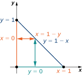
A sketch of the region appears in Figure 11.
We can complete this integration in two different ways.
- One way to look at it is by first integrating \(y\) from \(y=0\,\text{to}\,y=1-x\) vertically and then integrating \(x\) from \(x=0\,\text{to}\,x=1\text{:}\)
\[\begin{array}{ll}\underset{R}{∬}f(x,y)dx\,dy & =\int_{x=0}^{x=1}\,\int_{y=0}^{y=1-x}(x-2y)dy\,dx=\int_{x=0}^{x=1}{[xy-{y}^{2}]}_{y=0}^{y=1-x}dx \\ & =\int_{x=0}^{x=1}[x(1-x)-{(1-x)}^{2}]dx=\int_{x=0}^{x=1}[-1+3x-2{x}^{2}]dx={[\text{-}x+\frac{3}{2}{x}^{2}-\frac{2}{3}{x}^{3}]}_{x=0}^{x=1}=-\frac{1}{6}.\end{array}\]
- The other way to do this problem is by first integrating \(x\) from \(x=0\,\text{to}\,x=1-y\) horizontally and then integrating \(y\) from \(y=0\,\text{to}\,y=1\text{:}\)
\[\begin{array}{ll}\underset{R}{∬}f(x,y)dx\,dy & =\int_{y=0}^{y=1}\,\int_{x=0}^{x=1-y}(x-2y)dx\,dy=\int_{y=0}^{y=1}{[\frac{1}{2}{x}^{2}-2xy]}_{x=0}^{x=1-y}dy \\ & =\int_{y=0}^{y=1}[\frac{1}{2}{(1-y)}^{2}-2y(1-y)]dy=\int_{y=0}^{y=1}[\frac{1}{2}-3y+\frac{5}{2}{y}^{2}]dy \\ & ={[\frac{1}{2}y-\frac{3}{2}{y}^{2}+\frac{5}{6}{y}^{3}]}_{y=0}^{y=1}=-\frac{1}{6}.\end{array}\]
Evaluate the iterated integral \(\underset{D}{∬}({x}^{2}+{y}^{2})dA\) over the region \(D\) in the first quadrant between the functions \(y=2x\) and \(y={x}^{2}.\) Evaluate the iterated integral by integrating first with respect to \(y\) and then integrating first with resect to \(x.\)
\(\frac{216}{35}\)
Calculating Volumes, Areas, and Average Values
We can use double integrals over general regions to compute volumes, areas, and average values. The methods are the same as those in Double Integrals over Rectangular Regions, but without the restriction to a rectangular region, we can now solve a wider variety of problems.
Find the volume of the solid bounded by the planes \(x=0,y=0,z=0,\) and \(2x+3y+z=6.\)
Identify the base region D as Type I (or Type II), bounded by x=0, y=0, and 2x+3y=6, then integrate the height function 6-2x-3y over it.
The solid is a tetrahedron with the base on the \(xy\) -plane and a height \(z=6-2x-3y.\) The base is the region \(D\) bounded by the lines, \(x=0,y=0\) and \(2x+3y=6\) where \(z=0\) (Figure 12). Note that we can consider the region \(D\) as Type I or as Type II, and we can integrate in both ways.
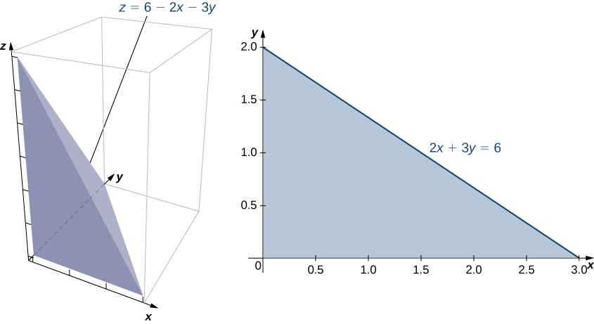
First, consider \(D\) as a Type I region, and hence \(D=\{(x,y)|0\le x\le 3,0\le y\le 2-\frac{2}{3}x\}.\)
Therefore, the volume is
\[\begin{array}{ll}V & =\int_{x=0}^{x=3}\,\int_{y=0}^{y=2-(2x\text{/}3)}(6-2x-3y)dy\,dx=\int_{x=0}^{x=3}[{(6y-2xy-\frac{3}{2}{y}^{2})|}_{y=0}^{y=2-(2x\text{/}3)}]dx \\ & =\int_{x=0}^{x=3}[\frac{2}{3}{(x-3)}^{2}]dx=6.\end{array}\]
Now consider \(D\) as a Type II region, so \(D=\{(x,y)|0\le y\le 2,0\le x\le 3-\frac{3}{2}y\}.\) In this calculation, the volume is
\[\begin{array}{ll}V & =\int_{y=0}^{y=2}\,\int_{x=0}^{x=3-(3y\text{/}2)}(6-2x-3y)dx\,dy=\int_{y=0}^{y=2}[{(6x-{x}^{2}-3xy)|}_{x=0}^{x=3-(3y\text{/}2)}]dy \\ & =\int_{y=0}^{y=2}[\frac{9}{4}{(y-2)}^{2}]dy=6.\end{array}\]
Therefore, the volume is \(6\) cubic units.
Find the volume of the solid bounded above by \(f(x,y)=10-2x+y\) over the region enclosed by the curves \(y=0\) and \(y={e}^{x},\) where \(x\) is in the interval \([0,1].\)
\(\frac{{e}^{2}}{4}+10e-\frac{49}{4}\) cubic units
Finding the area of a rectangular region is easy, but finding the area of a nonrectangular region is not so easy. As we have seen, we can use double integrals to find a rectangular area. As a matter of fact, this comes in very handy for finding the area of a general nonrectangular region, as stated in the next definition.
The area of a plane-bounded region \(D\) is defined as the double integral \(\underset{D}{∬}1dA.\)
We have already seen how to find areas in terms of single integration. Here we are seeing another way of finding areas by using double integrals, which can be very useful, as we will see in the later sections of this chapter.
Find the area of the region bounded below by the curve \(y={x}^{2}\) and above by the line \(y=2x\) in the first quadrant (Figure 13).
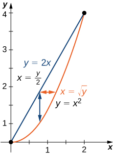
Set up the double integral of the constant function 1 over the region bounded by y=x² and y=2x.
We just have to integrate the constant function \(f(x,y)=1\) over the region. Thus, the area \(A\) of the bounded region is \(\int_{x=0}^{x=2}\,\int_{y={x}^{2}}^{y=2x}dy\,dx\) or \(\int_{y=0}^{y=4}\,\int_{x=y\text{/}2}^{x=\sqrt{y}}dx\,dy\text{:}\)
\[A=\underset{D}{∬}1dx\,dy=\int_{x=0}^{x=2}\,\int_{y={x}^{2}}^{y=2x}1dy\,dx=\int_{x=0}^{x=2}[{y|}_{y={x}^{2}}^{y=2x}]dx=\int_{x=0}^{x=2}(2x-{x}^{2})dx={{x}^{2}-\frac{{x}^{3}}{3}|}_{0}^{2}=\frac{4}{3}.\]
Find the area of a region bounded above by the curve \(y={x}^{3}\) and below by \(y=0\) over the interval \([0,3].\)
\(\frac{81}{4}\) square units
We can also use a double integral to find the average value of a function over a general region. The definition is a direct extension of the earlier formula.
If \(f(x,y)\) is integrable over a plane-bounded region \(D\) with positive area \(A(D),\) then the average value of the function is
\[{f}_{ave}=\frac{1}{A(D)}\underset{D}{∬}f(x,y)dA.\]
Note that the area is \(A(D)=\underset{D}{∬}1dA.\)
Find the average value of the function \(f(x,y)=7x{y}^{2}\) on the region bounded by the line \(x=y\) and the curve \(x=\sqrt{y}\) (Figure 14).
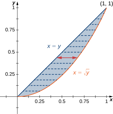
First compute the area A(D) by integrating 1 over the region, then divide the integral of f by that area.
First find the area \(A(D)\) where the region \(D\) is given by the figure. We have
\[A(D)=\underset{D}{∬}1dA=\int_{y=0}^{y=1}\,\int_{x=y}^{x=\sqrt{y}}1dx\,dy=\int_{y=0}^{y=1}[{x|}_{x=y}^{x=\sqrt{y}}]dy=\int_{y=0}^{y=1}(\sqrt{y}-y)dy=\frac{2}{3}{y}^{3\text{/}2}-{\frac{{y}^{2}}{2}|}_{0}^{1}=\frac{1}{6}.\]
Then the average value of the given function over this region is
\[\begin{array}{ll}{f}_{ave} & =\frac{1}{A(D)}\underset{D}{∬}f(x,y)dA=\frac{1}{A(D)}\int_{y=0}^{y=1}\,\int_{x=y}^{x=\sqrt{y}}7x{y}^{2}dx\,dy=\frac{1}{1\text{/}6}\int_{y=0}^{y=1}[{\frac{7}{2}{x}^{2}{y}^{2}|}_{x=y}^{x=\sqrt{y}}]dy \\ & =6\int_{y=0}^{y=1}[\frac{7}{2}{y}^{2}(y-{y}^{2})]dy=6\int_{y=0}^{y=1}[\frac{7}{2}({y}^{3}-{y}^{4})]dy=\frac{42}{2}{(\frac{{y}^{4}}{4}-\frac{{y}^{5}}{5})|}_{0}^{1}=\frac{42}{40}=\frac{21}{20}.\end{array}\]
Find the average value of the function \(f(x,y)=xy\) over the triangle with vertices \((0,0),(1,0)\,\text{and}\,(1,3).\)
\(\frac{3}{4}\)
Improper Double Integrals
An improper double integral is an integral \(\underset{D}{∬}f\,dA\) where either \(D\) is an unbounded region or \(f\) is an unbounded function. For example, \(D=\{(x,y)||x-y|\ge 2\}\) is an unbounded region, and the function \(f(x,y)=1\text{/}(1-{x}^{2}-2{y}^{2})\) over the ellipse \({x}^{2}+2{y}^{2}\le 1\) is an unbounded function. Hence, both of the following integrals are improper integrals:
- \(\underset{D}{∬}xy\,dA\) where \(D=\{(x,y)||x-y|\ge 2\};\)
- \(\underset{D}{∬}\frac{1}{1-{x}^{2}-2{y}^{2}}dA\) where \(D=\{(x,y)|{x}^{2}+2{y}^{2}\le 1\}.\)
In this section we would like to deal with improper integrals of functions over rectangles or simple regions such that \(f\) has only finitely many discontinuities. Not all such improper integrals can be evaluated; however, a form of Fubini’s theorem does apply for some types of improper integrals.
If \(D\) is a bounded rectangle or simple region in the plane defined by \(\{(x,y)\text{:}\,a\le x\le b,g(x)\le y\le h(x)\}\) and also by \(\{(x,y)\text{:}\,c\le y\le d,j(y)\le x\le k(y)\}\) and \(f\) is a nonnegative function on \(D\) with finitely many discontinuities in the interior of \(D,\) then
\[\underset{D}{∬}f\,dA=\int_{x=a}^{x=b}\,\int_{y=g(x)}^{y=h(x)}f(x,y)dy\,dx=\int_{y=c}^{y=d}\,\int_{x=j(y)}^{x=k(y)}f(x,y)dx\,dy.\]
It is very important to note that we required that the function be nonnegative on \(D\) for the theorem to work. We consider only the case where the function has finitely many discontinuities inside \(D.\)
Consider the function \(f(x,y)=\frac{{e}^{y}}{y}\) over the region \(D=\{(x,y)\text{:}\,0\le x\le 1,x\le y\le \sqrt{x}\}.\)
Notice that the function is nonnegative and continuous at all points on \(D\) except \((0,0).\) Use Fubini’s theorem to evaluate the improper integral.
Rewrite D as a Type II region so the integration order avoids the discontinuity at the origin, then apply Fubini's theorem for improper integrals.
First we plot the region \(D\) (Figure 15); then we express it in another way.
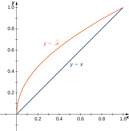
The other way to express the same region \(D\) is
\[D=\{(x,y)\text{:}\,0\le y\le 1,{y}^{2}\le x\le y\}.\]
Thus we can use Fubini’s theorem for improper integrals and evaluate the integral as
\[\int_{y=0}^{y=1}\,\int_{x={y}^{2}}^{x=y}\frac{{e}^{y}}{y}dx\,dy.\]
Therefore, we have
\[\int_{y=0}^{y=1}\,\int_{x={y}^{2}}^{x=y}\frac{{e}^{y}}{y}dx\,dy=\int_{y=0}^{y=1}\frac{{e}^{y}}{y}{x|}_{x={y}^{2}}^{x=y}dy=\int_{y=0}^{y=1}\frac{{e}^{y}}{y}(y-{y}^{2})dy=\int_{0}^{1}({e}^{y}-y{e}^{y})dy=e-2.\]
As mentioned before, we also have an improper integral if the region of integration is unbounded. Suppose now that the function \(f\) is continuous in an unbounded rectangle \(R.\)
If \(R\) is an unbounded rectangle such as \(R=\{(x,y)\text{:}\,a\le x<\infty ,c\le y<\infty \},\) then when the limit exists, we have \(\underset{R}{∬}f(x,y)dA=\underset{(b,d)\to (\infty ,\infty )}{\text{lim}}\int_{a}^{b}(\int_{c}^{d}f(x,y)dy)dx=\underset{(b,d)\to (\infty ,\infty )}{\text{lim}}\int_{c}^{d}(\int_{a}^{b}f(x,y)dx)dy.\)
The following example shows how this theorem can be used in certain cases of improper integrals.
Evaluate the integral \(\underset{R}{∬}xy{e}^{\text{-}{x}^{2}-{y}^{2}}dA\) where \(R\) is the first quadrant of the plane.
Replace the unbounded limits with variables b and d, evaluate the resulting iterated integral, then take the limit as b, d go to infinity.
The region \(R\) is the first quadrant of the plane, which is unbounded. So
\[\begin{array}{ll}\underset{R}{∬}xy{e}^{\text{-}{x}^{2}-{y}^{2}}dA & =\underset{(b,d)\to (\infty ,\infty )}{\text{lim}}\int_{x=0}^{x=b}(\int_{y=0}^{y=d}xy{e}^{\text{-}{x}^{2}-{y}^{2}}dy)dx=\underset{(b,d)\to (\infty ,\infty )}{\text{lim}}\int_{y=0}^{y=d}(\int_{x=0}^{x=b}xy{e}^{\text{-}{x}^{2}-{y}^{2}}dx)dy \\ & =\underset{(b,d)\to (\infty ,\infty )}{\text{lim}}\frac{1}{4}(1-{e}^{\text{-}{b}^{2}})(1-{e}^{\text{-}{d}^{2}})=\frac{1}{4}\end{array}\]
Thus, \(\underset{R}{∬}xy{e}^{\text{-}{x}^{2}-{y}^{2}}dA\) is convergent and the value is \(\frac{1}{4}.\)
Evaluate the improper integral \(\underset{D}{∬}\frac{y}{\sqrt{1-{x}^{2}-{y}^{2}}}dA\) where \(D=\{(x,y)|x\ge 0,y\ge 0,{x}^{2}+{y}^{2}\le 1\}.\)
\(\frac{\pi }{4}\)
In some situations in probability theory, we can gain insight into a problem when we are able to use double integrals over general regions. Before we go over an example with a double integral, we need to set a few definitions and become familiar with some important properties.
Consider a pair of continuous random variables \(X\) and \(Y,\) such as the birthdays of two people or the number of sunny and rainy days in a month. The joint density function \(f\) of \(X\) and \(Y\) satisfies the probability that \((X,Y)\) lies in a certain region \(D\text{:}\)
\[P((X,Y)\in D)=\underset{D}{∬}f(x,y)dA.\]
Since the probabilities can never be negative and must lie between \(0\) and \(1,\) the joint density function satisfies the following inequality and equation:
\[f(x,y)\ge 0\,\text{and}\,\underset{{R}^{2}}{∬}f(x,y)dA=1.\]
The variables \(X\) and \(Y\) are said to be independent random variables if their joint density function is the product of their individual density functions:
\[f(x,y)={f}_{1}(x){f}_{2}(y).\]
At Sydney’s Restaurant, customers must wait an average of \(15\) minutes for a table. From the time they are seated until they have finished their meal requires an additional \(40\) minutes, on average. What is the probability that a customer spends less than an hour and a half at the diner, assuming that waiting for a table and completing the meal are independent events?
Build the joint density function as the product of the two independent exponential densities, then integrate it over the triangular region x+y≤90.
Waiting times are mathematically modeled by exponential density functions, with \(m\) being the average waiting time, as
\[f(t)=\left\{\begin{array}{ll}0 & \text{if}\,t<0, \\ \frac{1}{m}{e}^{\text{-}t\text{/}m} & \text{if}\,t\ge 0.\end{array}\right.\]
If \(X\) and \(Y\) are random variables for ‘waiting for a table’ and ‘completing the meal,’ then the probability density functions are, respectively,
\[{f}_{1}(x)=\left\{\begin{array}{ll}0 & \text{if}\,x<0, \\ \frac{1}{15}{e}^{\text{-}x\text{/}15} & \text{if}\,x\ge 0.\end{array}\right.\,\text{and}\,{f}_{2}(y)=\left\{\begin{array}{ll}0 & \text{if}\,y<0, \\ \frac{1}{40}{e}^{\text{-}y\text{/}40} & \text{if}\,y\ge 0.\end{array}\right.\]
Clearly, the events are independent and hence the joint density function is the product of the individual functions
\[f(x,y)={f}_{1}(x){f}_{2}(y)=\left\{\begin{array}{ll}0 & \text{if}\,x<0\,\text{or}\,y<0, \\ \frac{1}{600}{e}^{\text{-}x\text{/}15}{e}^{\text{-}y\text{/}60} & \text{if}\,x,y\ge 0.\end{array}\right.\]
We want to find the probability that the combined time \(X+Y\) is less than \(90\) minutes. In terms of geometry, it means that the region \(D\) is in the first quadrant bounded by the line \(x+y=90\) (Figure 16).
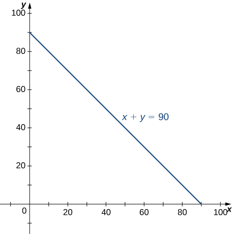
Hence, the probability that \((X,Y)\) is in the region \(D\) is
\[P(X+Y\le 90)=P((X,Y)\in D)=\underset{D}{∬}f(x,y)dA=\underset{D}{∬}\frac{1}{600}{e}^{\text{-}x\text{/}15}{e}^{\text{-}y\text{/}40}dA.\]
Since \(x+y=90\) is the same as \(y=90-x,\) we have a region of Type I, so
\[\begin{array}{lll}D & = & \{(x,y)|0\le x\le 90,0\le y\le 90-x\}, \\ P(X+Y\le 90) & = & \begin{array}{ll}\frac{1}{600} & \int_{x=0}^{x=90}\int_{y=0}^{y=90-x}{e}^{\text{-}x\text{/}15}{e}^{\text{-}y\text{/}40}dy dx\end{array} \\ & = & \begin{array}{ll}\frac{1}{600} & \int_{x=0}^{x=90}\int_{y=0}^{y=90-x}{e}^{\text{-}(x\text{/}15+y\text{/}40)}dy dx=0.8328.\end{array}\end{array}\]
Thus, there is an \(83.28\text{\%}\) chance that a customer spends less than an hour and a half at the restaurant.
Another important application in probability that can involve improper double integrals is the calculation of expected values. First we define this concept and then show an example of a calculation.
In probability theory, we denote the expected values \(E(X)\) and \(E(Y),\) respectively, as the most likely outcomes of the events. The expected values \(E(X)\) and \(E(Y)\) are given by
\[E(X)=\underset{S}{∬}xf(x,y)dA\,\text{and}\,E(Y)=\underset{S}{∬}yf(x,y)dA,\]
where \(S\) is the sample space of the random variables \(X\) and \(Y.\)
Find the expected time for the events ‘waiting for a table’ and ‘completing the meal’ in Example 12.
Set up the improper double integral for E(X) using the joint density from the restaurant example, and evaluate it as a product of two one-variable limits.
Using the first quadrant of the rectangular coordinate plane as the sample space, we have improper integrals for \(E(X)\) and \(E(Y).\) The expected time for a table is
\[\begin{array}{ll}E(X) & =\underset{S}{∬}x\frac{1}{600}{e}^{\text{-}x\text{/}15}{e}^{\text{-}y\text{/}40}dA=\frac{1}{600}\int_{x=0}^{x=\infty} \,\int_{y=0}^{y=\infty} x{e}^{\text{-}x\text{/}15}{e}^{\text{-}y\text{/}40}dA \\ & =\frac{1}{600}\underset{(a,b)\to (\infty ,\infty )}{\text{lim}}\int_{x=0}^{x=a}\,\int_{y=0}^{y=b}x{e}^{\text{-}x\text{/}15}{e}^{\text{-}y\text{/}40}dx\,dy \\ & =\frac{1}{600}(\underset{a\to \infty }{\text{lim}}\int_{x=0}^{x=a}x{e}^{\text{-}x\text{/}15}dx)(\underset{b\to \infty }{\text{lim}}\int_{y=0}^{y=b}{e}^{\text{-}y\text{/}40}dy) \\ & =\frac{1}{600}({(\underset{a\to \infty }{\text{lim}}(-15{e}^{\text{-}x\text{/}15}(x+15)))|}_{x=0}^{x=a})({(\underset{b\to \infty }{\text{lim}}(-40{e}^{\text{-}y\text{/}40}))|}_{y=0}^{y=b}) \\ & =\frac{1}{600}(\underset{a\to \infty }{\text{lim}}(-15{e}^{\text{-}a\text{/}15}(x+15)+225))(\underset{b\to \infty }{\text{lim}}(-40{e}^{\text{-}b\text{/}40}+40)) \\ & =\frac{1}{600}(225)(40) \\ & =15.\end{array}\]
A similar calculation shows that \(E(Y)=40.\) This means that the expected values of the two random events are the average waiting time and the average dining time, respectively.
The joint density function for two random variables \(X\) and \(Y\) is given by
\[f(x,y)=\begin{array}{ll}\frac{1}{16250}({x}^{2}+{y}^{2}) & \text{if}\,0\le x\le 15,0\le y\le 10 \\ 0 & \text{otherwise}\end{array}\]
Find the probability that \(X\) is at most \(10\) and \(Y\) is at least \(5.\)
\(\frac{11}{39}\approx 0.282\)
Key Concepts
- A general bounded region \(D\) on the plane is a region that can be enclosed inside a rectangular region. We can use this idea to define a double integral over a general bounded region. (See Example 1.)
- To evaluate an iterated integral of a function over a general nonrectangular region, we sketch the region and express it as a Type I or as a Type II region or as a union of several Type I or Type II regions that overlap only on their boundaries. (See Example 2, Example 3, and Example 4.)
- We can use double integrals to find volumes, areas, and average values of a function over general regions, similarly to calculations over rectangular regions. (See Example 7, Example 8, and Example 9.)
- We can use Fubini’s theorem for improper integrals to evaluate some types of improper integrals. (See Example 10 and Example 11.)
Key Equations
| Iterated integral over a Type I region | \(\underset{D}{∬}f(x,y)dA=\underset{D}{∬}f(x,y)dy\,dx=\int_{a}^{b}[\int_{{g}_{1}(x)}^{{g}_{2}(x)}f(x,y)dy]dx\) |
| Iterated integral over a Type II region | \(\underset{D}{∬}f(x,y)dA=\underset{D}{∬}f(x,y)dx\,dy=\int_{c}^{d}[\int_{{h}_{1}(y)}^{{h}_{2}(y)}f(x,y)dx]dy\) |
Section Exercises
In the following exercises, specify whether the region is of Type I or Type II.
The region \(D\) bounded by \(y={x}^{3},\) \(y={x}^{3}+1,\) \(x=0,\) and \(x=1\) as given in the following figure.
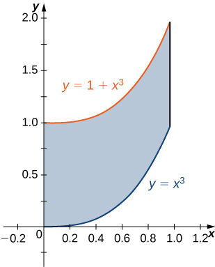
Find the average value of the function \(f(x,y)=3xy\) on the region graphed in the previous exercise.
\(\frac{27}{20}\)
Find the area of the region \(D\) given in the previous exercise.
The region \(D\) bounded by \(y=\text{sin}\,x,y=1+\text{sin}\,x,x=0,\,\text{and}\,x=\frac{\pi }{2}\) as given in the following figure.
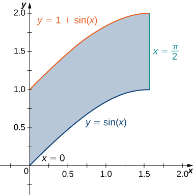
Type I but not Type II
Find the average value of the function \(f(x,y)=\text{cos}\,x\) on the region graphed in the previous exercise.
Find the area of the region \(D\) given in the previous exercise.
\(\frac{\pi }{2}\)
The region \(D\) bounded by \(x={y}^{2}-1\) and \(x=\sqrt{1-{y}^{2}}\) as given in the following figure.
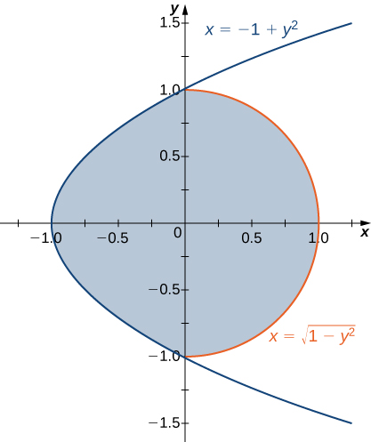
Find the volume of the solid under the graph of the function \(f(x,y)=xy+1\) and above the region in the figure in the previous exercise.
\(\frac{1}{6}(8+3\pi )\)
The region \(D\) bounded by \(y=0,x=-10+y,\,\text{and}\,x=10-y\) as given in the following figure.
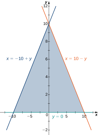
Find the signed volume of the solid under the graph of the function \(f(x,y)=x+y\) and above the region in the figure from the previous exercise.
\(\frac{1000}{3}\)
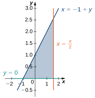
The region \(D\) bounded by \(y=0,x=y-1,\) \(x=\frac{\pi }{2}\) as given in the following figure.
The region \(D\) bounded by \(y=0\) and \(y={x}^{2}-1\) as given in the following figure.
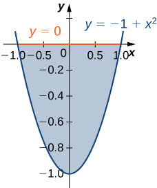
Type I and Type II
Let \(D\) be the region bounded by the curve \(y=2-{x}^{2}\) and below the equations \(y=x,y=\text{-}x,\) Explain why \(D\) is neither of Type I nor II.
Let \(D\) be the region bounded above by the curve of the equation \(y=4-{x}^{2}\) and below by \(y=\text{cos}x\) and the \(x\) -axis. Explain why \(D\) is neither of Type I nor II.
The region \(D\) is not of Type I: it does not lie between two vertical lines and the graphs of two continuous functions \({g}_{1}(x)\) and \({g}_{2}(x).\) The region \(D\) is not of Type II: it does not lie between two horizontal lines and the graphs of two continuous functions \({h}_{1}(y)\) and \({h}_{2}(y).\)
In the following exercises, evaluate the double integral \(\underset{D}{∬}f(x,y)dA\) over the region \(D.\)
\(f(x,y)=2x+5y\) and \(D=\{(x,y)|0\le x\le 1,{x}^{3}\le y\le {x}^{3}+1\}\)
\(f(x,y)=1\) and \(D=\{(x,y)|0\le x\le \frac{\pi }{2},\text{sin}\,x\le y\le 1+\text{sin}\,x\}\)
\(\frac{\pi }{2}\)
\(f(x,y)=2\) and \(D=\{(x,y)|0\le y\le 1,y-1\le x\le \text{arccos}\,y\}\)
\(f(x,y)=xy\) and \(D=\{(x,y)|-1\le y\le 1,{y}^{2}-1\le x\le \sqrt{1-{y}^{2}}\}\)
\(0\)
\(f(x,y)=\text{sin}\,y\) and \(D\) is the triangular region with vertices \((0,0),(0,3),\,\text{and}\,(3,0)\)
\(f(x,y)=\text{-}x+1\) and \(D\) is the triangular region with vertices \((0,0),(0,2),\,\text{and}\,(2,2)\)
\(\frac{2}{3}\)
Evaluate the iterated integrals.
\(\int_{0}^{1}\,\int_{2x}^{3x}(x+{y}^{2})dy\,dx\)
\(\int_{0}^{1}\,\int_{2\sqrt{x}}^{2\sqrt{x}+1}(xy+1)dy\,dx\)
\(\frac{41}{20}\)
\(\int_{e}^{{e}^{2}}\,\int_{\text{ln}\,u}^{2}(v+\text{ln}\,u)dv\,du\)
\(\int_{1}^{2}\,\int_{\text{-}{u}^{2}-1}^{\text{-}u}(8uv)dv\,du\)
\(-63\)
\(\int_{0}^{1}\,\int_{\text{-}\sqrt{1-{y}^{2}}}^{\sqrt{1-{y}^{2}}}(2x+4{x}^{3})dx\,dy\)
\(\int_{0}^{1\text{/}2}\,\int_{\text{-}\sqrt{1-4{y}^{2}}}^{\sqrt{1-4{y}^{2}}}4dx\,dy\)
\(\pi\)
Let \(D\) be the region in the first quadrant bounded by \(y=1-{x}^{2},y=4-{x}^{2},\) and the \(x\) - and \(y\) -axes.
- Show that \(\underset{D}{∬}x\,dA=\int_{0}^{1}\,\int_{1-{x}^{2}}^{4-{x}^{2}}x\,dy\,dx+\int_{1}^{2}\,\int_{0}^{4-{x}^{2}}x\,dy\,dx\) by dividing the region \(D\) into two regions of Type I.
- Evaluate the integral \(\underset{D}{∬}x\,dA.\)
Let \(D\) be the region bounded by \(y=1,\) \(y=x,\) \(y=\text{ln}\,x,\) and the \(x\) -axis.
- Show that \(\underset{D}{∬}y\,dA=\int_{0}^{1}\,\int_{0}^{x}y\,dy\,dx+\int_{1}^{e}\,\int_{\text{ln}\,x}^{1}y\,dy\,dx\) by dividing \(D\) into two regions of Type I.
- Evaluate the integral \(\underset{D}{∬}y\,dA.\)
a. Answers may vary; b. \(\frac{2}{3}\)
- Show that \(\underset{D}{∬}{y}^{2}dA=\int_{-1}^{0}\,\int_{\text{-}x}^{2-{x}^{2}}{y}^{2}dy\,dx+\int_{0}^{1}\,\int_{x}^{2-{x}^{2}}{y}^{2}dy\,dx\) by dividing the region \(D\) into two regions of Type I, where \(D=\{(x,y)|y\ge x,y\ge -x,y\le 2-{x}^{2}\}.\)
- Evaluate the integral \(\underset{D}{∬}{y}^{2}dA.\)
Let \(D\) be the region bounded by \(y={x}^{2},y=x+2,\) and \(y=\text{-}x.\)
- Show that \(\underset{D}{∬}x\,dA=\int_{0}^{1}\,\int_{\text{-}y}^{\sqrt{y}}x\,dx\,dy+\int_{1}^{4}\,\int_{y-2}^{\sqrt{y}}x\,dx\,dy\) by dividing the region \(D\) into two regions of Type II, where \(D=\{(x,y)|y\ge {x}^{2},y\ge -x,y\le x+2\}.\)
- Evaluate the integral \(\underset{D}{∬}x\,dA.\)
a. Answers may vary; b. \(\frac{7}{3}\)
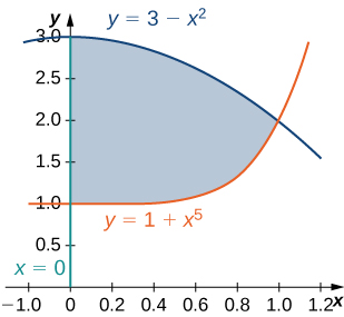
The region \(D\) bounded by \(x=0,y={x}^{5}+1,\) and \(y=3-{x}^{2}\) is shown in the following figure. Find the area \(A(D)\) of the region \(D.\)
The region \(D\) bounded by \(y=\text{cos}\,x,y=4+\text{cos}\,x,\) and \(x=\pm \frac{\pi }{3}\) is shown in the following figure. Find the area \(A(D)\) of the region \(D.\)
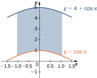
\(\frac{8\pi }{3}\)
Find the area \(A(D)\) of the region \(D=\{(x,y)|y\ge 1-{x}^{2},y\le 4-{x}^{2},y\ge 0,x\ge 0\}.\)
Let \(D\) be the region bounded by \(y=1,y=x,y=\text{ln}\,x,\) and the \(x\) -axis. Find the area \(A(D)\) of the region \(D.\)
\(e-\frac{3}{2}\)
Find the average value of the function \(f(x,y)=\text{sin}\,y\) on the triangular region with vertices \((0,0),(0,3),\) and \((3,0).\)
Find the average value of the function \(f(x,y)=\text{-}x+1\) on the triangular region with vertices \((0,0),(0,2),\) and \((2,2).\)
\(\frac{1}{3}\)
In the following exercises, change the order of integration and evaluate the integral.
\(\int_{-1}^{\pi \text{/}2}\,\int_{0}^{x+1}\text{sin}\,x\,dy\,dx\)
\(\int_{0}^{1}\,\int_{x-1}^{1-x}x\,dy\,dx\)
\(\int_{0}^{1}\,\int_{x-1}^{1-x}x\,dy\,dx=\int_{-1}^{0}\,\int_{0}^{y+1}x\,dx\,dy+\int_{0}^{1}\,\int_{0}^{1-y}x\,dxdy=\frac{1}{3}\)
\(\int_{-1}^{0}\,\int_{\text{-}\sqrt{y+1}}^{\sqrt{y+1}}{y}^{2}dx\,dy\)
\(\int_{\text{-1}}^{1}\,\int_{\text{-}\sqrt{1-{y}^{2}}}^{\sqrt{1-{y}^{2}}}y\,dx\,dy\)
\(\int_{\text{-1}}^{1}\,\int_{\text{-}\sqrt{1-{y}^{2}}}^{\sqrt{1-{y}^{2}}}y\,dx\,dy=\int_{\text{-1}}^{1}\,\int_{\text{-}\sqrt{1-{x}^{2}}}^{\sqrt{1-{x}^{2}}}y\,dy\,dx=0\)
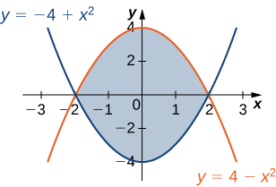
The region \(D\) is shown in the following figure. Evaluate the double integral \(\underset{D}{∬}({x}^{2}+y)dA\) by using the easier order of integration.
The region \(D\) is given in the following figure. Evaluate the double integral \(\underset{D}{∬}({x}^{2}-{y}^{2})dA\) by using the easier order of integration.
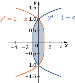
\(\underset{D}{∬}({x}^{2}-{y}^{2})dA=\int_{-1}^{1}\,\int_{{y}^{4}-1}^{1-{y}^{4}}({x}^{2}-{y}^{2})dx\,dy=\frac{464}{4095}\)
Find the volume of the solid under the surface \(z=2x+{y}^{2}\) and above the region bounded by \(y={x}^{5}\) and \(y=x.\)
Find the volume in the first octant of the solid under the plane \(z=3x+y\) and above the region determined by \(y={x}^{7}\) and \(y=x.\)
\(\frac{4}{5}\)
Find the volume of the solid under the plane \(z=x-y\) and above the region bounded by \(x=\text{tan}\,y,x=\text{-}\text{tan}\,y,\) and \(x=1.\)
Find the volume of the solid under the surface \(z={x}^{3}\) and above the plane region bounded by \(x=\text{sin}\,y,x=\text{-}\text{sin}\,y,\) and \(x=1\) for values of \(y\) between \(y=\frac{-\pi }{2}\,\text{ and }\,y=\frac{\pi }{2}\)
\(\frac{5\pi }{32}\)
Let \(g\) be a positive, increasing, and differentiable function on the interval \([a,b].\) Show that the volume of the solid under the surface \(z=g\prime (x)\) and above the region bounded by \(y=0,\) \(y=g(x),\) \(x=a,\) and \(x=b\) is given by \(\frac{1}{2}({g}^{2}(b)-{g}^{2}(a)).\)
Let \(g\) be a positive, increasing, and differentiable function on the interval \([a,b],\) and let \(k\) be a positive real number. Show that the volume of the solid under the surface \(z=g\prime (x)\) and above the region bounded by \(y=g(x),y=g(x)+k,x=a,\) and \(x=b\) is given by \(k(g(b)-g(a)).\)
Find the volume of the solid situated in the first octant and determined by the planes \(z=2,\) \(z=0,x+y=1,x=0,\,\text{and}\,y=0.\)
Find the volume of the solid situated in the first octant and bounded by the planes \(x+2y=1,\) \(x=0,y=0,z=4,\,\text{and}\,z=0.\)
\(1\)
Find the volume of the solid bounded by the planes \(x+y=1,x-y=1,x=0,z=0,\) and \(z=10.\)
Find the volume of the solid bounded by the planes \(x+y=1,x-y=1,x+y=-1,\) \(x-y=-1,z=1\,\text{and}\,z=0.\)
\(2\)
Let \({S}_{1}\) and \({S}_{2}\) be the solids situated in the first octant under the planes \(x+y+z=1\) and \(x+y+2z=1,\) respectively, and let \(S\) be the solid situated between \({S}_{1},{S}_{2},x=0,\,\text{and}\,y=0.\)
- Find the volume of the solid \({S}_{1}.\)
- Find the volume of the solid \({S}_{2}.\)
- Find the volume of the solid \(S\) by subtracting the volumes of the solids \({S}_{1}\,\text{and}\,{S}_{2}.\)
Let \({S}_{1}\,\text{and}\,{S}_{2}\) be the solids situated in the first octant under the planes \(2x+2y+z=2\) and \(x+y+z=1,\) respectively, and let \(S\) be the solid situated between \({S}_{1},{S}_{2},x=0,\,\text{and}\,y=0.\)
- Find the volume of the solid \({S}_{1}.\)
- Find the volume of the solid \({S}_{2}.\)
- Find the volume of the solid \(S\) by subtracting the volumes of the solids \({S}_{1}\,\text{and}\,{S}_{2}.\)
a. \(\frac{1}{3};\) b. \(\frac{1}{6};\) c. \(\frac{1}{6}\)
Let \({S}_{1}\,\text{and}\,{S}_{2}\) be the solids situated in the first octant under the plane \(x+y+z=2\) and under the sphere \({x}^{2}+{y}^{2}+{z}^{2}=4,\) respectively. If the volume of the solid \({S}_{2}\) is \(\frac{4\pi }{3},\) determine the volume of the solid \(S\) situated between \({S}_{1}\) and \({S}_{2}\) by subtracting the volumes of these solids.
Consider the plane \(x + y + z = 2\) and the cylinder \({x}^{2} + {y}^{2} = 4\) in the first octant.
- Find the volume under the plane.
- Find the volume inside the cylinder under the plane \(z = 2\) .
- Find the volume above the plane, inside the cylinder, and below the plane \(z = 2\) .
a. \(\frac{4}{3};\) b. \(2\pi ;\) c. \(\frac{6\pi -4}{3}\)
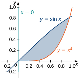
[T] The following figure shows the region \(D\) bounded by the curves \(y=\text{sin}\,x,\) \(x=0,\) and \(y={x}^{4}.\) Use a graphing calculator or CAS to find the \(x\) -coordinates of the intersection points of the curves and to determine the area of the region \(D.\) Round your answers to six decimal places.
[T] The region \(D\) bounded by the curves \(y=\text{cos}\,x,x=0,\,\text{and}\,y={x}^{3}\) is shown in the following figure. Use a graphing calculator or CAS to find the x-coordinates of the intersection points of the curves and to determine the area of the region \(D.\) Round your answers to six decimal places.
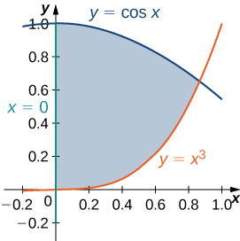
\(0\,\text{and}\,0.865474;\) \(A(D)=0.621135\)
Suppose that \((X,Y)\) is the outcome of an experiment that must occur in a particular region \(S\) in the \(xy\) -plane. In this context, the region \(S\) is called the sample space of the experiment and \(X\,\text{and}\,Y\) are random variables. If \(D\) is a region included in \(S,\) then the probability of \((X,Y)\) being in \(D\) is defined as \(P[(X,Y)\in D]=\underset{D}{∬}p(x,y)dx\,dy,\) where \(p(x,y)\) is the joint probability density of the experiment. Here, \(p(x,y)\) is a nonnegative function for which \(\underset{S}{∬}p(x,y)dx\,dy=1.\) Assume that a point \((X,Y)\) is chosen arbitrarily in the square \([0,3]\,\times \,[0,3]\) with the probability density
\(p(x,y)=\left\{\begin{array}{ll}\frac{1}{9} & (x,y)\in [0,3]\,\times \,[0,3], \\ 0 & \text{otherwise}\text{.}\end{array}\right.\)
Find the probability that the point \((X,Y)\) is inside the unit square and interpret the result.
Consider \(X\,\text{and}\,Y\) two random variables of probability densities \({p}_{1}(x)\) and \({p}_{2}(y),\) respectively. The random variables \(X\,\text{and}\,Y\) are said to be independent if their joint density function is given by \(p(x,y)={p}_{1}(x){p}_{2}(y).\) At a drive-thru restaurant, customers spend, on average, \(3\) minutes placing their orders and an additional \(5\) minutes paying for and picking up their meals. Assume that placing the order and paying for/picking up the meal are two independent events \(X\) and \(Y.\) If the waiting times are modeled by the exponential probability densities
\(\begin{array}{lllllll}{p}_{1}(x)=\left\{\begin{array}{ll}\frac{1}{3}{e}^{\text{-}x\text{/}3} & x\ge 0, \\ 0 & \text{otherwise,}\end{array}\right. & & & \text{and} & & & {p}_{2}(y)=\left\{\begin{array}{ll}\frac{1}{5}{e}^{\text{-}y\text{/}5} & y\ge 0, \\ 0 & \text{otherwise,}\end{array}\right.\end{array}\)
respectively, the probability that a customer will spend less than 6 minutes in the drive-thru line is given by \(P[X+Y\le 6]=\underset{D}{∬}p(x,y)dx\,dy,\) where \(D=\{(x,y)\}|x\ge 0,y\ge 0,x+y\le 6\}.\) Find \(P[X+Y\le 6]\) and interpret the result.
\(P[X+Y\le 6]=1+\frac{3}{2{e}^{2}}-\frac{5}{{e}^{6\text{/}5}}\approx 0.45;\) there is a \(45\text{\%}\) chance that a customer will spend \(6\) minutes in the drive-thru line.
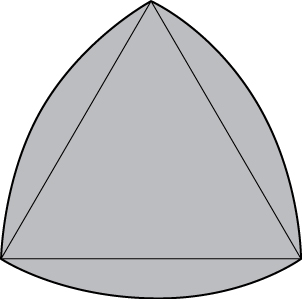
[T] The Reuleaux triangle consists of an equilateral triangle and three regions, each of them bounded by a side of the triangle and an arc of a circle of radius s centered at the opposite vertex of the triangle. Show that the area of the Reuleaux triangle in the following figure of side length \(s\) is \(\frac{{s}^{2}}{2}(\pi -\sqrt{3}).\)
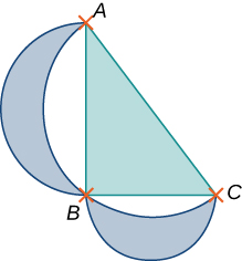
[T] Show that the area of the lunes of Alhazen, the two blue lunes in the following figure, is the same as the area of the right triangle ABC. The outer boundaries of the lunes are semicircles of diameters \(AB\,\text{and}\,BC,\) respectively, and the inner boundaries are formed by the circumcircle of the triangle \(ABC.\)
Glossary
- improper double integral
- a double integral over an unbounded region or of an unbounded function
- Type I
- a region \(D\) in the \(xy\) -plane is Type I if it lies between two vertical lines and the graphs of two continuous functions \({g}_{1}(x)\) and \({g}_{2}(x)\)
- Type II
- a region \(D\) in the \(xy\) -plane is Type II if it lies between two horizontal lines and the graphs of two continuous functions \({h}_{1}(y)\,\text{and}\,{h}_{2}(y)\)