Section 5.1Double Integrals over Rectangular Regions
In this section we investigate double integrals and show how we can use them to find the volume of a solid over a rectangular region in the \(xy\) -plane. Many of the properties of double integrals are similar to those we have already discussed for single integrals.
Volumes and Double Integrals
We begin by considering the space above a rectangular region R. Consider a continuous function \(f(x,y)\ge 0\) of two variables defined on the closed rectangle R:
\[R=[a,b]\,\times \,[c,d]=\left\{(x,y)\in {ℝ}^{2}|a\le x\le b,c\le y\le d\}\right.\]
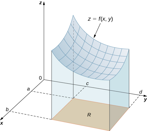
Here \([a,b]\,\times \,[c,d]\) denotes the Cartesian product of the two closed intervals \([a,b]\) and \([c,d].\) It consists of rectangular pairs \((x,y)\) such that \(a\le x\le b\) and \(c\le y\le d.\) The graph of \(f\) represents a surface above the \(xy\) -plane with equation \(z=f(x,y)\) where \(z\) is the height of the surface at the point \((x,y).\) Let \(S\) be the solid that lies above \(R\) and under the graph of \(f\) (Figure 1). The base of the solid is the rectangle \(R\) in the \(xy\) -plane. We want to find the volume \(V\) of the solid \(S.\)
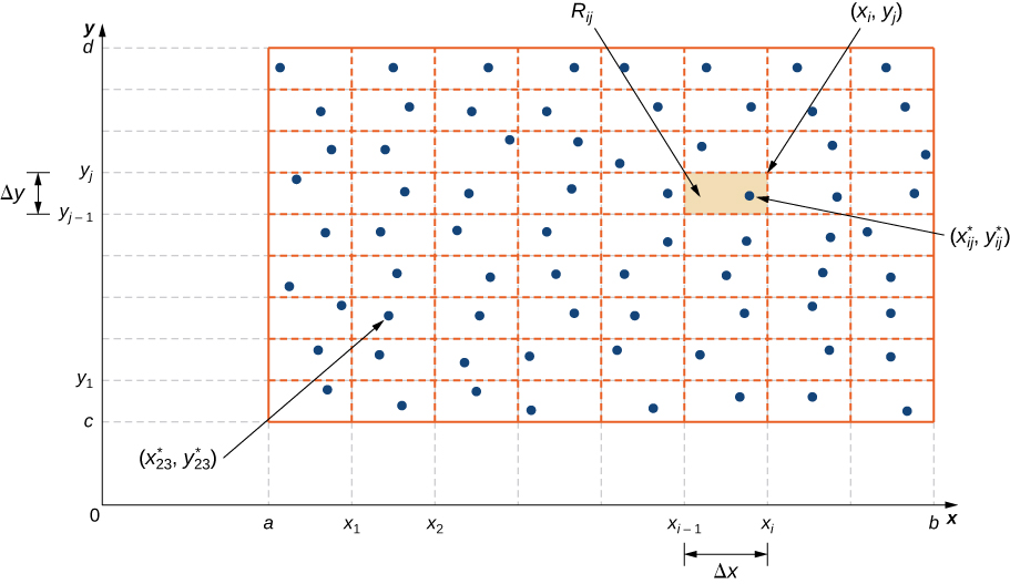
We divide the region \(R\) into small rectangles \({R}_{ij},\) each with area \(\Delta A\) and with sides \(\Delta x\) and \(\Delta y\) (Figure 2). We do this by dividing the interval \([a,b]\) into \(m\) subintervals and dividing the interval \([c,d]\) into \(n\) subintervals. Hence \(\Delta x=\frac{b-a}{m},\) \(\Delta y=\frac{d-c}{n},\) and \(\Delta A=\Delta x\Delta y.\)
The volume of a thin rectangular box above \({R}_{ij}\) is \(f({x}_{ij}^{*},{y}_{ij}^{*})\Delta A,\) where \(({x}_{ij}^{*},{y}_{ij}^{*})\) is an arbitrary sample point in each \({R}_{ij}\) as shown in the following figure.
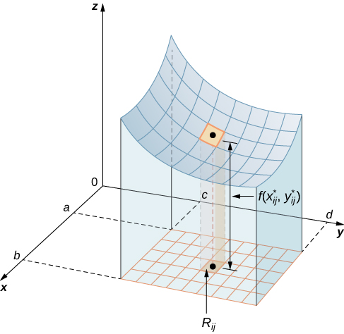
Using the same idea for all the subrectangles, we obtain an approximate volume of the solid \(S\) as \(V\approx \sum_{i=1}^{m}\sum_{j=1}^{n}f({x}_{ij}^{*},{y}_{ij}^{*})\Delta A.\) This sum is known as a double Riemann sum and can be used to approximate the value of the volume of the solid. Here the double sum means that for each subrectangle we evaluate the function at the chosen point, multiply by the area of each rectangle, and then add all the results.
As we have seen in the single-variable case, we obtain a better approximation to the actual volume if m and n become larger.
\[V=\underset{m,n\to \infty }{\text{lim}}\sum_{i=1}^{m}\sum_{j=1}^{n}f({x}_{ij}^{*},{y}_{ij}^{*})\Delta A\,\text{or}\,V=\underset{\Delta x,\Delta y\to 0}{\text{lim}}\sum_{i=1}^{m}\sum_{j=1}^{n}f({x}_{ij}^{*},{y}_{ij}^{*})\Delta A.\]
Note that the sum approaches a limit in either case and the limit is the volume of the solid with the base R. Now we are ready to define the double integral.
The double integral of the function \(f(x,y)\) over the rectangular region \(R\) in the \(xy\) -plane is defined as
\[\underset{R}{∬}f(x,y)dA=\underset{m,n\to \infty }{\text{lim}}\sum_{i=1}^{m}\sum_{j=1}^{n}f({x}_{i}^{*},{y}_{j}^{*})\Delta A.\]
If \(f(x,y)\ge 0,\) then the volume V of the solid S, which lies above \(R\) in the \(xy\) -plane and under the graph of f, is the double integral of the function \(f(x,y)\) over the rectangle \(R.\) If the function is ever negative, then the double integral can be considered a “signed” volume in a manner similar to the way we defined net signed area in The Definite Integral.
Consider the function \(z=f(x,y)=3{x}^{2}-y\) over the rectangular region \(R=[0,2]\,\times \,[0,2]\) (Figure 4).
- Set up a double integral for finding the value of the signed volume of the solid S that lies above \(R\) and “under” the graph of \(f.\)
- Divide R into four squares with \(m=n=2,\) and choose the sample point as the upper right corner point of each square \((1,1),(2,1),(1,2),\) and \((2,2)\) (Figure 5) to approximate the signed volume of the solid S that lies above \(R\) and “under” the graph of \(f.\)
- Divide R into four squares with \(m=n=2,\) and choose the sample point as the midpoint of each square: \((1\text{/}2,1\text{/}2),(3\text{/}2,1\text{/}2),(1\text{/}2,3\text{/}2),\text{and}\,(3\text{/}2,3\text{/}2)\) to approximate the signed volume.
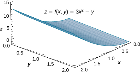
Figure 4 — The function \(z=f(x,y)\) graphed over the rectangular region \(R=[0,2]\,\times \,[0,2].\)
Start by writing the definition of the double integral as a limit of Riemann sums, then plug in each set of sample points in turn.
- As we can see, the function \(z=f(x,y)=3{x}^{2}-y\) is both above and below the plane. To find the signed volume of S, we need to divide the region R into small rectangles \({R}_{ij},\) each with area \(\Delta A\) and with sides \(\Delta x\) and \(\Delta y,\) and choose \(({x}_{ij}^{*},{y}_{ij}^{*})\) as sample points in each \({R}_{ij}.\) Hence, a double integral is set up as
\[V=\underset{R}{∬}(3{x}^{2}-y)dA=\underset{m,n\to \infty }{\text{lim}}\sum_{i=1}^{m}\sum_{j=1}^{n}[3{({x}_{ij}^{*})}^{2}-{y}_{ij}^{*}]\Delta A.\]
- Approximating the signed volume using a Riemann sum with \(m=n=2\) we have \(\Delta A=\Delta x\Delta y=1\,\times \,1=1.\) Also, the sample points are (1, 1), (2, 1), (1, 2), and (2, 2) as shown in the following figure.
Hence,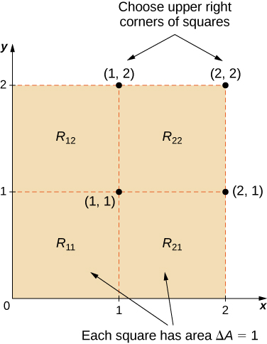
Figure 5 — Subrectangles for the rectangular region \(R=[0,2]\,\times \,[0,2].\) \[\begin{array}{ll}V & =\sum_{i=1}^{2}\sum_{j=1}^{2}f({x}_{ij}^{*},{y}_{ij}^{*})\Delta A \\ & =\sum_{i=1}^{2}(f({x}_{i1}^{*},{y}_{i1}^{*})+f({x}_{i2}^{*},{y}_{i2}^{*}))\Delta A \\ & =f({x}_{11}^{*},{y}_{11}^{*})\Delta A+f({x}_{21}^{*},{y}_{21}^{*})\Delta A+f({x}_{12}^{*},{y}_{12}^{*})\Delta A+f({x}_{22}^{*},{y}_{22}^{*})\Delta A \\ & =f(1,1)(1)+f(2,1)(1)+f(1,2)(1)+f(2,2)(1) \\ & =\left(3-1\right)(1)+(12-1)(1)+(3-2)(1)+(12-2)(1) \\ & =2 + 11 + 1 + 10 = 24\end{array}\]
- Approximating the signed volume using a Riemann sum with \(m=n=2,\) we have \(\Delta A=\Delta x\Delta y=1\,\times \,1=1.\) In this case the sample points are (1/2, 1/2), (3/2, 1/2), (1/2, 3/2),
and (3/2, 3/2).
Hence\[\begin{array}{ll}V & =\sum_{i=1}^{2}\sum_{j=1}^{2}f({x}_{ij}^{*},{y}_{ij}^{*})\Delta A \\ & =f({x}_{11}^{*},{y}_{11}^{*})\Delta A+f({x}_{21}^{*},{y}_{21}^{*})\Delta A+f({x}_{12}^{*},{y}_{12}^{*})\Delta A+f({x}_{22}^{*},{y}_{22}^{*})\Delta A \\ & =f(\frac{1}{2},\frac{1}{2})(1)+f(\frac{3}{2},\frac{1}{2})(1)+f(\frac{1}{2},\frac{3}{2})(1)+f(\frac{3}{2},\frac{3}{2})(1) \\ & =(\frac{3}{4}-\frac{1}{2})(1)+(\frac{27}{4}-\frac{1}{2})(1)+(\frac{3}{4}-\frac{3}{2})(1)+(\frac{27}{4}-\frac{3}{2})(1) \\ & =\frac{1}{4}+\frac{25}{4}+(-\frac{3}{4})+\frac{21}{4}=\frac{44}{4}\end{array}\]
Notice that the approximate answers differ due to the choices of the sample points. In either case, we are introducing some error because we are using only a few sample points. Thus, we need to investigate how we can achieve an accurate answer.
Use the same function \(z=f(x,y)=3{x}^{2}-y\) over the rectangular region \(R=[0,2]\,\times \,[0,2].\)
Divide R into the same four squares with \(m=n=2,\) and choose the sample points as the upper left corner point of each square \((0,1),(1,1),(0,2),\) and \((1,2)\) (Figure 5) to approximate the signed volume of the solid S that lies above \(R\) and “under” the graph of \(f.\)
\(V=\sum_{i=1}^{2}\sum_{j=1}^{2}f({x}_{ij}^{*},{y}_{ij}^{*})\Delta A=0\)
Note that we developed the concept of double integral using a rectangular region R. This concept can be extended to any general region. However, when a region is not rectangular, the subrectangles may not all fit perfectly into R, particularly if the base area is curved. We examine this situation in more detail in the next section, where we study regions that are not always rectangular and subrectangles may not fit perfectly in the region R. Also, the heights may not be exact if the surface \(z=f(x,y)\) is curved. However, the errors on the sides and the height where the pieces may not fit perfectly within the solid S approach 0 as m and n approach infinity. Also, the double integral of the function \(z=f(x,y)\) exists provided that the function \(f\) is not too discontinuous. If the function is bounded and continuous over R except on a finite number of smooth curves, then the double integral exists and we say that \(f\) is integrable over R.
Since \(\Delta A=\Delta x\Delta y=\Delta y\Delta x,\) we can express \(dA\) as \(dx\,dy\) or \(dy\,dx.\) This means that, when we are using rectangular coordinates, the double integral over a region \(R\) denoted by \(\underset{R}{∬}f(x,y)dA\) can be written as \(\underset{R}{∬}f(x,y)dx\,dy\) or \(\underset{R}{∬}f(x,y)dy\,dx.\)
Now let’s list some of the properties that can be helpful to compute double integrals.
Properties of Double Integrals
The properties of double integrals are very helpful when computing them or otherwise working with them. We list here six properties of double integrals. Properties 1 and 2 are referred to as the linearity of the integral, property 3 is the additivity of the integral, property 4 is the monotonicity of the integral, and property 5 is used to find the bounds of the integral. Property 6 is used if \(f(x,y)\) is a product of two functions \(g(x)\) and \(h(y).\)
Assume that the functions \(f(x,y)\) and \(g(x,y)\) are integrable over the rectangular region R; S and T are subregions of R; and assume that m and M are real numbers.
- The sum \(f(x,y)+g(x,y)\) is integrable and
\[\underset{R}{∬}[f(x,y)+g(x,y)]dA=\underset{R}{∬}f(x,y)dA+\underset{R}{∬}g(x,y)dA.\]
- If c is a constant, then \(cf(x,y)\) is integrable and
\[\underset{R}{∬}cf(x,y)dA=c\underset{R}{∬}f(x,y)dA.\]
- If \(R=S∪T\) and \(S∩T=\varnothing\) except an overlap on the boundaries, then
\[\underset{R}{∬}f(x,y)dA=\underset{S}{∬}f(x,y)dA+\underset{T}{∬}f(x,y)dA.\]
- If \(f(x,y)\ge g(x,y)\) for \((x,y)\) in \(R,\) then
\[\underset{R}{∬}f(x,y)dA\ge \underset{R}{∬}g(x,y)dA.\]
- If \(m\le f(x,y)\le M,\) then
\[m\,\times \,A(R)\le \underset{R}{∬}f(x,y)dA\le M\,\times \,A(R).\]
- In the case where \(f(x,y)\) can be factored as a product of a function \(g(x)\) of \(x\) only and a function \(h(y)\) of \(y\) only, then over the region \(R=\{(x,y)|a\le x\le b,c\le y\le d\},\) the double integral can be written as
\[\underset{R}{∬}f(x,y)dA=({∫}_{a}^{b}g(x)dx)({∫}_{c}^{d}h(y)dy).\]
These properties are used in the evaluation of double integrals, as we will see later. We will become skilled in using these properties once we become familiar with the computational tools of double integrals. So let’s get to that now.
Iterated Integrals
So far, we have seen how to set up a double integral and how to obtain an approximate value for it. We can also imagine that evaluating double integrals by using the definition can be a very lengthy process if we choose larger values for \(m\) and \(n.\) Therefore, we need a practical and convenient technique for computing double integrals. In other words, we need to learn how to compute double integrals without employing the definition that uses limits and double sums.
The basic idea is that the evaluation becomes easier if we can break a double integral into single integrals by integrating first with respect to one variable and then with respect to the other. The key tool we need is called an iterated integral.
Assume \(a,b,c,\) and \(d\) are real numbers. We define an iterated integral for a function \(f(x,y)\) over the rectangular region \(R\) \(=[a,b]\,\times \,[c,d]\) as
\[\int_{a}^{b}\,\int_{c}^{d}f(x,y)dy\,dx=\int_{a}^{b}[\int_{c}^{d}f(x,y)dy]dx\]
\[\int_{c}^{d}\,\int_{a}^{b}f(x,y)dx\,dy=\int_{c}^{d}[\int_{a}^{b}f(x,y)dx]dy.\]
The notation \(\int_{a}^{b}[\int_{c}^{d}f(x,y)dy]dx\) means that we integrate \(f(x,y)\) with respect to y while holding x constant. Similarly, the notation \(\int_{c}^{d}[\int_{a}^{b}f(x,y)dx]dy\) means that we integrate \(f(x,y)\) with respect to x while holding y constant. The fact that double integrals can be split into iterated integrals is expressed in Fubini’s theorem. Think of this theorem as an essential tool for evaluating double integrals.
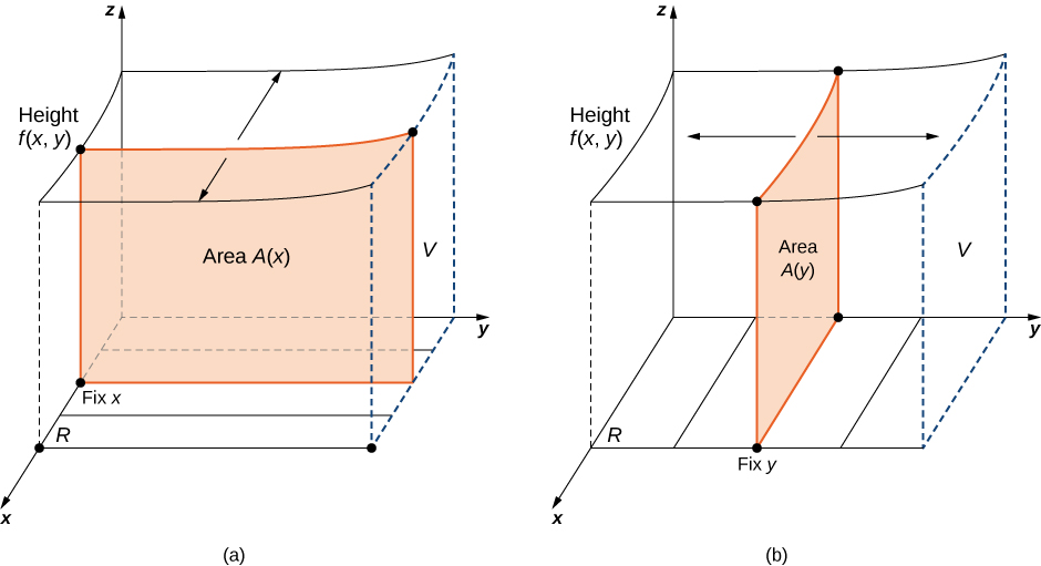
Suppose that \(f(x,y)\) is a function of two variables that is continuous over a rectangular region \(R=\{(x,y)\in {ℝ}^{2}|a\le x\le b,\text{c}\le \text{y}\le \text{d}\}.\) Then we see from Figure 6 that the double integral of \(f\) over the region equals an iterated integral,
\[\underset{R}{∬}f(x,y)dA=\underset{R}{∬}f(x,y)dx\,dy=\int_{a}^{b}\,\int_{c}^{d}f(x,y)dy\,dx=\int_{c}^{d}\,\int_{a}^{b}f(x,y)dx\,dy.\]
More generally, Fubini’s theorem is true if \(f\) is bounded on \(R\) and \(f\) is discontinuous only on a finite number of continuous curves. In other words, \(f\) has to be integrable over \(R.\)
Use Fubini’s theorem to compute the double integral \(\underset{R}{∬}f(x,y)dA\) where \(f(x,y)=x\) and \(R=[0,2]\,\times \,[0,1].\)
Convert the double integral to an iterated integral using Fubini's theorem, integrating with respect to x first.
Fubini’s theorem offers an easier way to evaluate the double integral by the use of an iterated integral. Note how the boundary values of the region R become the upper and lower limits of integration.
\[\begin{array}{ll}\underset{R}{∬}f(x,y)dA & =\underset{R}{∬}f(x,y)dx\,dy \\ & ={∫}_{y=0}^{y=1}{∫}_{x=0}^{x=2}x\,dx\,dy \\ & ={∫}_{y=0}^{y=1}[{\frac{{x}^{2}}{2}|}_{x=0}^{x=2}]dy \\ & ={∫}_{y=0}^{y=1}2dy={2y|}_{y=0}^{y=1}=2.\end{array}\]
The double integration in this example is simple enough to use Fubini’s theorem directly, allowing us to convert a double integral into an iterated integral. Consequently, we are now ready to convert all double integrals to iterated integrals and demonstrate how the properties listed earlier can help us evaluate double integrals when the function \(f(x,y)\) is more complex. Note that the order of integration can be changed (see Example 7).
Evaluate the double integral \(\underset{R}{∬}(xy-3x{y}^{2})dA\) where \(R=\{(x,y)|0\le x\le 2,1\le y\le 2\}.\)
Split the integrand into two pieces using linearity, then convert each piece to an iterated integral.
This function has two pieces: one piece is \(xy\) and the other is \(3x{y}^{2}.\) Also, the second piece has a constant \(3.\) Notice how we use properties i and ii to help evaluate the double integral.
\[\begin{array}{llll} \\ \\ \\ \\ \,\underset{R}{∬}(xy-3x{y}^{2})dA & & & \\ =\underset{R}{∬}xy\,dA+\underset{R}{∬}(-3x{y}^{2})dA & & & \text{Property i: Integral of a sum is the sum of the integrals.} \\ ={∫}_{y=1}^{y=2}{∫}_{x=0}^{x=2}xy\,dx\,dy-{∫}_{y=1}^{y=2}{∫}_{x=0}^{x=2}3x{y}^{2}dx\,dy & & & \text{Convert double integrals to iterated integrals.} \\ ={∫}_{y=1}^{y=2}{(\frac{{x}^{2}}{2}y)|}_{x=0}^{x=2}dy-3{∫}_{y=1}^{y=2}{(\frac{{x}^{2}}{2}{y}^{2})|}_{x=0}^{x=2}dy & & & \text{Integrate with respect to}\,x,\text{holding}\,y\,\text{constant.} \\ ={∫}_{y=1}^{y=2}2y\,dy-{∫}_{y=1}^{y=2}6{y}^{2}dy & & & \text{Property ii: Placing the constant before the integral.} \\ =2{∫}_{1}^{2}y\,dy-6{∫}_{1}^{2}{y}^{2}dy & & & \text{Integrate with respect to}\,y. \\ ={2\frac{{y}^{2}}{2}|}_{1}^{2}-{6\frac{{y}^{3}}{3}|}_{1}^{2} & & & \\ ={{y}^{2}|}_{1}^{2}-{2{y}^{3}|}_{1}^{2} & & & \\ =(4-1)-2(8-1) & & & \\ =3-2(7)=3-14=-11.\end{array}\]
Over the region \(R=\{(x,y)|1\le x\le 3,1\le y\le 2\},\) we have \(2\le {x}^{2}+{y}^{2}\le 13.\) Find a lower and an upper bound for the integral \(\underset{R}{∬}({x}^{2}+{y}^{2})dA.\)
Use the boundedness property, integrating the constant lower bound and the constant upper bound separately over R.
For a lower bound, integrate the constant function 2 over the region \(R.\) For an upper bound, integrate the constant function 13 over the region \(R.\)
\[\begin{array}{lll}{∫}_{1}^{2}{∫}_{1}^{3}2dx\,dy & = & {∫}_{1}^{2}[{2x|}_{1}^{3}]dy={∫}_{1}^{2}2(2)dy={4y|}_{1}^{2}=4(2-1)=4 \\ {∫}_{1}^{2}{∫}_{1}^{3}13dx\,dy & = & {∫}_{1}^{2}[{13x|}_{1}^{3}]dy={∫}_{1}^{2}13(2)dy={26y|}_{1}^{2}=26(2-1)=26.\end{array}\]
Hence, we obtain \(4\le \underset{R}{∬}({x}^{2}+{y}^{2})dA\le 26.\)
Evaluate the integral \(\underset{R}{∬}{e}^{y}\text{cos}\,x\,dA\) over the region \(R=\{(x,y)|0\le x\le \frac{\pi }{2},0\le y\le 1\}.\)
Recognize the integrand factors into a function of x times a function of y, then split the double integral into a product of two single integrals.
This is a great example for property vi because the function \(f(x,y)\) is clearly the product of two single-variable functions \({e}^{y}\) and \(\text{cos}\,x.\) Thus we can split the integral into two parts and then integrate each one as a single-variable integration problem.
\[\begin{array}{ll}\underset{R}{∬}{e}^{y}\text{cos}\,x\,dA & ={∫}_{0}^{1}{∫}_{0}^{\pi \text{/}2}{e}^{y}\text{cos}\,x\,dx\,dy \\ & =({∫}_{0}^{1}{e}^{y}dy)({∫}_{0}^{\pi \text{/}2}\text{cos}\,x\,dx) \\ & =({{e}^{y}|}_{0}^{1})({\text{sin}\,x|}_{0}^{\pi \text{/}2}) \\ & =e-1.\end{array}\]
- Use the properties of the double integral and Fubini’s theorem to evaluate the integral
\[{∫}_{0}^{1}{∫}_{-1}^{3}(3-x+4y)dy\,dx.\]
- Show that \(0\le \underset{R}{∬}\text{sin}\,\pi x\,\text{cos}\,\pi y\,dA\le \frac{1}{32}\) where \(R=\left(0,\frac{1}{4}\right)\times \left(\frac{1}{4},\frac{1}{2}\right).\)
a. 26 b. Answers may vary.
As we mentioned before, when we are using rectangular coordinates, the double integral over a region \(R\) denoted by \(\underset{R}{∬}f(x,y)dA\) can be written as \(\underset{R}{∬}f(x,y)dx\,dy\) or \(\underset{R}{∬}f(x,y)dy\,dx.\) The next example shows that the results are the same regardless of which order of integration we choose.
Let’s return to the function \(f(x,y)=3{x}^{2}-y\) from Example 1, this time over the rectangular region \(R=[0,2]\,\times \,[0,3].\) Use Fubini’s theorem to evaluate \(\underset{R}{∬}f(x,y)dA\) in two different ways:
- First integrate with respect to y and then with respect to x;
- First integrate with respect to x and then with respect to y.
Set up the iterated integral both ways — y first then x, and x first then y — using the boundary values of R as the limits.
Figure 6 shows how the calculation works in two different ways.
- First integrate with respect to y and then integrate with respect to x:
\[\begin{array}{ll}\underset{R}{∬}f(x,y)dA & ={∫}_{x=0}^{x=2}{∫}_{y=0}^{y=3}(3{x}^{2}-y)dy\,dx \\ & ={∫}_{x=0}^{x=2}(\int_{y=0}^{y=3}(3{x}^{2}-y)dy)dx={∫}_{x=0}^{x=2}[{3{x}^{2}y-\frac{{y}^{2}}{2}|}_{y=0}^{y=3}]dx \\ & ={∫}_{x=0}^{x=2}(9{x}^{2}-\frac{9}{2})dx={3{x}^{3}-\frac{9}{2}x|}_{x=0}^{x=2}=15.\end{array}\]
- First integrate with respect to x and then integrate with respect to y:
\[\begin{array}{ll}\underset{R}{∬}f(x,y)dA & ={∫}_{y=0}^{y=3}{∫}_{x=0}^{x=2}(3{x}^{2}-y)dx\,dy \\ & ={∫}_{y=0}^{y=3}({∫}_{x=0}^{x=2}(3{x}^{2}-y)dx)dy={∫}_{y=0}^{y=3}[{{x}^{3}-xy|}_{x=0}^{x=2}]dy \\ & ={∫}_{y=0}^{y=3}(8-2y)dy={8y-{y}^{2}|}_{y=0}^{y=3}=15.\end{array}\]
With either order of integration, the double integral gives us an answer of 15. We might wish to interpret this answer as a volume in cubic units of the solid \(S\) below the function \(f(x,y)=3{x}^{2}-y\) over the region \(R=[0,2]\,\times \,[0,3].\) However, remember that the interpretation of a double integral as a (non-signed) volume works only when the integrand \(f\) is a nonnegative function over the base region \(R.\)
Evaluate \({∫}_{y=-3}^{y=2}{∫}_{x=3}^{x=5}(2-3{x}^{2}+{y}^{2})dx\,dy.\)
\(-\frac{1340}{3}\)
In the next example we see that it can actually be beneficial to switch the order of integration to make the computation easier. We will come back to this idea several times in this chapter.
Consider the double integral \(\underset{R}{∬}x\,\text{sin}(xy)dA\) over the region \(R=\{(x,y)|0\le x\le \pi ,1\le y\le 2\}\) (Figure 7).
- Express the double integral in two different ways.
- Analyze whether evaluating the double integral in one way is easier than the other and why.
- Evaluate the integral.
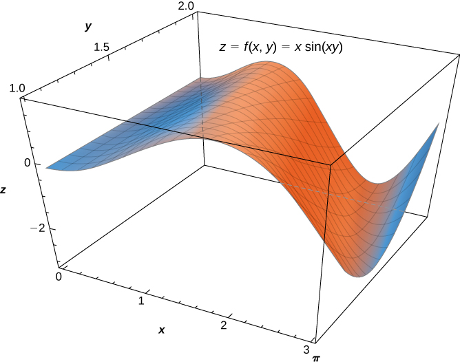
Figure 7 — The function \(z=f(x,y)=x\,\text{sin}(xy)\) over the rectangular region \(R=[0,\pi ]\,\times \,[1,2].\)
Write the integral both orders and compare; integrating y first turns into a quick substitution while x first requires integration by parts.
- We can express \(\underset{R}{∬}x\,\text{sin}(xy)dA\) in the following two ways: first by integrating with respect to \(y\) and then with respect to \(x;\) second by integrating with respect to \(x\) and then with respect to \(y.\)
\[\begin{array}{llll} \\ \\ \\ \\ \,\underset{R}{∬}x\,\text{sin}(xy)dA & & & \\ =\int_{x=0}^{x=\pi} \,\int_{y=1}^{y=2}x\,\text{sin}(xy)dy\,dx & & & \text{Integrate first with respect to}\,y. \\ =\int_{y=1}^{y=2}\,\int_{x=0}^{x=\pi} x\,\text{sin}(xy)dx\,dy & & & \text{Integrate first with respect to}\,x.\end{array}\]
- If we want to integrate with respect to y first and then integrate with respect to \(x,\) we see that we can use the substitution \(u=xy,\) which gives \(du=x\,dy.\) Hence the inner integral is simply \(∫\text{sin}\,u\,du\) and we can change the limits to be functions of x,
However, integrating with respect to \(x\) first and then integrating with respect to \(y\) requires integration by parts for the inner integral, with \(u=x\) and \(dv=\text{sin}(xy)dx.\)
Then \(du=dx\) and \(v=-\frac{\text{cos}(xy)}{y},\) so
Since the evaluation is getting complicated, we will only do the computation that is easier to do, which is clearly the first method.\[\underset{R}{∬}x\,\text{sin}(xy)dA=\int_{x=0}^{x=\pi} \,\int_{y=1}^{y=2}x\,\text{sin}(xy)dy\,dx=\int_{x=0}^{x=\pi} [\int_{u=x}^{u=2x}\text{sin}(u)du]dx.\]
\[\underset{R}{∬}x\,\text{sin}(xy)dA=\int_{y=1}^{y=2}\,\int_{x=0}^{x=\pi} x\,\text{sin}(xy)dx\,dy=\int_{y=1}^{y=2}[-{\frac{x\,\text{cos}(xy)}{y}|}_{x=0}^{x=\pi }+\frac{1}{y}\int_{x=0}^{x=\pi} \text{cos}(xy)dx]dy.\]
- Evaluate the double integral using the easier way.
\[\begin{array}{ll}\underset{R}{∬}x\,\text{sin}(xy)dA & =\int_{x=0}^{x=\pi} \,\int_{y=1}^{y=2}x\,\text{sin}(xy)dy\,dx \\ & =\int_{x=0}^{x=\pi} [\int_{u=x}^{u=2x}\text{sin}(u)du]dx=\int_{x=0}^{x=\pi} [{\text{-}\text{cos}\,u|}_{u=x}^{u=2x}]dx=\int_{x=0}^{x=\pi} (\text{-}\text{cos}\,2x+\text{cos}\,x)dx \\ & ={-\frac{1}{2}\text{sin}\,2x+\text{sin}\,x|}_{x=0}^{x=\pi }=0.\end{array}\]
Evaluate the integral \(\underset{R}{∬}x{e}^{xy}dA\) where \(R=[0,1]\,\times \,[0,\text{ln}\,5].\)
\(\frac{4-\text{ln}\,5}{\text{ln}\,5}\)
Applications of Double Integrals
Double integrals are very useful for finding the area of a region bounded by curves of functions. We describe this situation in more detail in the next section. However, if the region is a rectangular shape, we can find its area by integrating the constant function \(f(x,y)=1\) over the region \(R.\)
The area of the region \(R\) is given by \(A(R)=\underset{R}{∬}1dA.\)
This definition makes sense because using \(f(x,y)=1\) and evaluating the integral make it a product of length and width. Let’s check this formula with an example and see how this works.
Find the area of the region \(R=\{(x,y)|0\le x\le 3,0\le y\le 2\}\) by using a double integral, that is, by integrating 1 over the region \(R.\)
Set up the double integral with integrand 1 over the region, since area equals the integral of the constant function 1.
The region is rectangular with length 3 and width 2, so we know that the area is 6. We get the same answer when we use a double integral:
\[A(R)=\int_{0}^{2}\,\int_{0}^{3}1dx\,dy=\int_{0}^{2}[{x|}_{0}^{3}]dy=\int_{0}^{2}3dy=3\int_{0}^{2}dy=3{y|}_{0}^{2}=3(2)=6.\]
We have already seen how double integrals can be used to find the volume of a solid bounded above by a function \(f(x,y)\) over a region \(R\) provided \(f(x,y)\ge 0\) for all \((x,y)\) in \(R.\) Here is another example to illustrate this concept.
Find the volume \(V\) of the solid \(S\) that is bounded by the elliptic paraboloid \(2{x}^{2}+{y}^{2}+z=27,\) the planes \(x=3\) and \(y=3,\) and the three coordinate planes.
Identify the region R2=[0,3]×[0,3] under the paraboloid and set up the double integral of z=27-2x²-y² over it.
First notice the graph of the surface \(z=27-2{x}^{2}-{y}^{2}\) in Figure 8(a) and above the square region \({R}_{1}=[-3,3]\,\times \,[-3,3].\) However, we need the volume of the solid bounded by the elliptic paraboloid \(2{x}^{2}+{y}^{2}+z=27,\) the planes \(x=3\) and \(y=3,\) and the three coordinate planes.
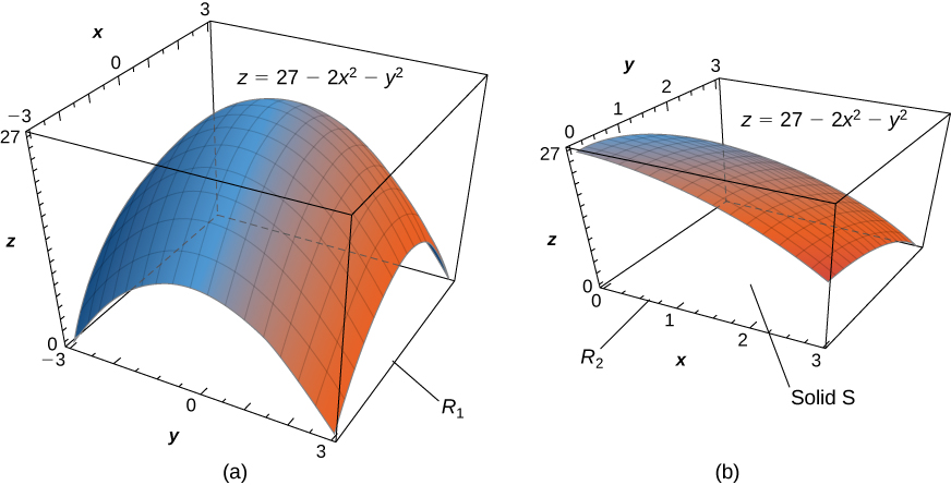
Now let’s look at the graph of the surface in Figure 8(b). We determine the volume V by evaluating the double integral over \({R}_{2}\text{:}\)
\[\begin{array}{lllll}V & =\underset{R}{∬}z\,dA=\underset{R}{∬}(27-2{x}^{2}-{y}^{2})dA & & & \\ & =\int_{y=0}^{y=3}\,\int_{x=0}^{x=3}(27-2{x}^{2}-{y}^{2})dx\,dy & & & \text{Convert to iterated integral.} \\ & =\int_{y=0}^{y=3}{[27x-\frac{2}{3}{x}^{3}-{y}^{2}x]|}_{x=0}^{x=3}dy & & & \text{Integrate with respect to}\,x. \\ & =\int_{y=0}^{y=3}(63-3{y}^{2})dy=63y-{{y}^{3}|}_{y=0}^{y=3}=162. & & & \end{array}\]
Find the volume of the solid bounded above by the graph of \(f(x,y)=xy\,\text{sin}({x}^{2}y)\) and below by the \(xy\) -plane on the rectangular region \(R=[0,1]\,\times \,[0,\pi ].\)
\(\frac{\pi }{2}\)
Recall that we defined the average value of a function of one variable on an interval \([a,b]\) as
\[{f}_{\text{ave}}=\frac{1}{b-a}\int_{a}^{b}f(x)dx.\]
Similarly, we can define the average value of a function of two variables over a region R. The main difference is that we divide by an area instead of the width of an interval.
The average value of a function of two variables over a region \(R\) is
\[{f}_{\text{ave}}=\frac{1}{\text{Area}\,R}\underset{R}{∬}f(x,y)dA.\]
In the next example we find the average value of a function over a rectangular region. This is a good example of obtaining useful information for an integration by making individual measurements over a grid, instead of trying to find an algebraic expression for a function.
The weather map in Figure 9 shows an unusually moist storm system associated with the remnants of Hurricane Karl, which dumped 4–8 inches (100–200 mm) of rain in some parts of the Midwest on September 22–23, 2010. The area of rainfall measured 300 miles east to west and 250 miles north to south. Estimate the average rainfall over the entire area in those two days.
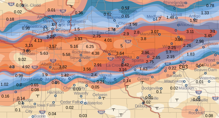
Divide the map into six subrectangles and read off the rainfall value at each midpoint to apply the average-value formula.
Place the origin at the southwest corner of the map so that all the values can be considered as being in the first quadrant and hence all are positive. Now divide the entire map into six rectangles \((m=3\,\text{and}\,n=2),\) as shown in Figure 10. Assume \(f(x,y)\) denotes the storm rainfall in inches at a point approximately \(x\) miles to the east of the origin and y miles to the north of the origin. Let \(R\) represent the entire area of \(250\,\times \,300=75000\) square miles. Then the area of each subrectangle is
\[\Delta A=\frac{1}{6}(75,000)=12,500.\]
Assume \(({x}_{ij}^{*},{y}_{ij}^{*})\) are approximately the midpoints of each subrectangle \({R}_{ij}.\) Note the color-coded region at each of these points, and estimate the rainfall. The rainfall at each of these points can be estimated as:
At \((x{*}_{11},y{*}_{11})\) the rainfall is 0.08.
At \((x{*}_{21},y{*}_{21})\) the rainfall is 0.08.
At \((x{*}_{31},y{*}_{31})\) the rainfall is 0.01.
At \((x{*}_{12},y{*}_{12})\) the rainfall is 1.70.
At \((x{*}_{22},y{*}_{22})\) the rainfall is 1.74.
At \((x{*}_{32},y{*}_{32})\) the rainfall is 3.00.
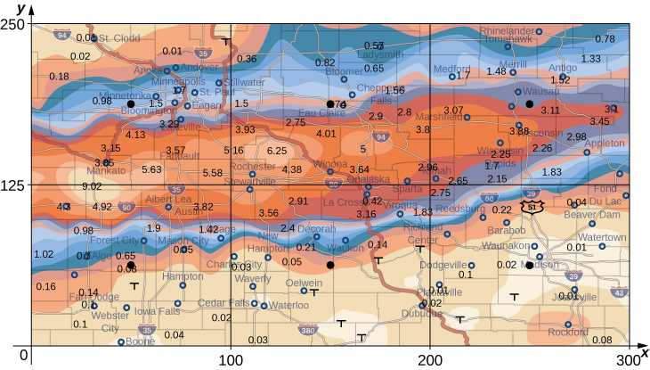
According to our definition, the average storm rainfall in the entire area during those two days was
\[\begin{array}{ll}{f}_{\text{ave}} & =\frac{1}{\text{Area}\,R}\underset{R}{∬}f(x,y)dx\,dy=\frac{1}{75000}\underset{R}{∬}f(x,y)dx\,dy \\ & \approx \frac{1}{75,000}\sum_{i=1}^{3}\sum_{j=1}^{2}f({x}_{ij}^{*},{y}_{ij}^{*})\Delta A \\ & \approx \frac{1}{75,000}[f({x}_{11}^{*},{y}_{11}^{*})\Delta A+f({x}_{21}^{*},{y}_{21}^{*})\Delta A \\ & \,+f({x}_{31}^{*},{y}_{31}^{*})\Delta A+f({x}_{12}^{*},{y}_{12}^{*})\Delta A+f({x}_{22}^{*},{y}_{22}^{*})\Delta A+f({x}_{32}^{*},{y}_{32}^{*})\Delta A] \\ & \approx \frac{1}{75,000}[0.08+0.08+0.01+1.70+1.74+3.00]\Delta A \\ & \approx \frac{1}{75,000}[0.08+0.08+0.01+1.70+1.74+3.00]12500 \\ & \approx \frac{5}{30}[0.08+0.08+0.01+1.70+1.74+3.00] \\ & \approx 1.10.\end{array}\]
During September 22–23, 2010 this area had an average storm rainfall of approximately 1.10 inches.
A contour map is shown for a function \(f(x,y)\) on the rectangle \(R=[-3,6]\,\times \,[-1,4].\)
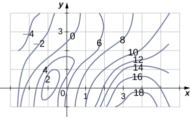
- Use the midpoint rule with \(m=3\) and \(n=2\) to estimate the value of \(\underset{R}{∬}f(x,y)dA.\)
- Estimate the average value of the function \(f(x,y).\)
Answers to both parts a. and b. may vary.
Key Concepts
- We can use a double Riemann sum to approximate the volume of a solid bounded above by a function of two variables over a rectangular region. By taking the limit, this becomes a double integral representing the volume of the solid. (See Example 1.)
- Properties of double integral are useful to simplify computation and find bounds on their values. (See Example 4 and Example 5.)
- We can use Fubini’s theorem to write and evaluate a double integral as an iterated integral. (See Example 2, Example 6, and Example 7.)
- Double integrals are used to calculate the area of a region, the volume under a surface, and the average value of a function of two variables over a rectangular region. (See Example 8, Example 9, and Example 10.)
Key Equations
| Double integral | \(\underset{R}{∬}f(x,y)dA=\underset{m,n\to \infty }{\text{lim}}\sum_{i=1}^{m}\sum_{j=1}^{n}f({x}_{ij}^{*},{y}_{ij}^{*})\Delta A\) |
| Iterated integral | \({∫}_{a}^{b}{∫}_{c}^{d}f(x,y)dx\,dy={∫}_{a}^{b}[{∫}_{c}^{d}f(x,y)dy]dx\) or \({∫}_{c}^{d}{∫}_{b}^{a}f(x,y)dx\,dy={∫}_{c}^{d}[{∫}_{a}^{b}f(x,y)dx]dy\) |
| Average value of a function of two variables | \({f}_{\text{ave}}=\frac{1}{\text{Area}\,R}\underset{R}{∬}f(x,y)dx\,dy\) |
Section Exercises
In the following exercises, use the midpoint rule with \(m=4\) and \(n=2\) to estimate the volume of the solid bounded by the surface \(z=f(x,y),\) the vertical planes \(x=1,\) \(x=2,\) \(y=1,\) and \(y=2,\) and the horizontal plane \(z=0.\)
\(f(x,y)=4x+2y+8xy\)
27.
\(f(x,y)=16{x}^{2}+\frac{y}{2}\)
In the following exercises, estimate \({∬}_{R}f\left(x,y\right)dA\) by using a Riemann sum with \(m=n=2\) and the sample points to be the lower left corners of the subrectangles of the partition.
\(f(x,y)=\text{sin}\,x-\text{cos}\,y,\) \(R=[0,\pi ]\,\times \,[0,\pi ]\)
0.
\(f(x,y)=\text{cos}\,x+\text{cos}\,y,\) \(R=[0,\pi ]\,\times \,[0,\frac{\pi }{2}]\)
Use the midpoint rule with \(m=n=2\) to estimate \(\underset{R}{∬}f(x,y)dA,\) where the values of the function f on \(R=[8,10]\,\times \,[9,11]\) are given in the following table.
| y | |||||
| x | 9 | 9.5 | 10 | 10.5 | 11 |
| 8 | 9.8 | 5 | 6.7 | 5 | 5.6 |
| 8.5 | 9.4 | 4.5 | 8 | 5.4 | 3.4 |
| 9 | 8.7 | 4.6 | 6 | 5.5 | 3.4 |
| 9.5 | 6.7 | 6 | 4.5 | 5.4 | 6.7 |
| 10 | 6.8 | 6.4 | 5.5 | 5.7 | 6.8 |
21.3.
The values of the function f on the rectangle \(R=[0,2]\,\times \,[7,9]\) are given in the following table. Estimate the double integral \(\underset{R}{∬}f(x,y)dA\) by using a Riemann sum with \(m=n=2.\) Select the sample points to be the upper right corners of the subsquares of R.
| \({y}_{0}=7\) | \({y}_{1}=8\) | \({y}_{2}=9\) | |
| \({x}_{0}=0\) | 10.22 | 10.21 | 9.85 |
| \({x}_{1}=1\) | 6.73 | 9.75 | 9.63 |
| \({x}_{2}=2\) | 5.62 | 7.83 | 8.21 |
The depth of a children’s 4-ft by 4-ft swimming pool, measured at 1-ft intervals, is given in the following table.
- Estimate the volume of water in the swimming pool by using a Riemann sum with \(m=n=2.\) Select the sample points using the midpoint rule on \(R=[0,4]\,\times \,[0,4].\)
- Approximate the average depth of the swimming pool.
Table 4 y x 0 1 2 3 4 0 1 1.5 2 2.5 3 1 1 1.5 2 2.5 3 2 1 1.5 1.5 2.5 3 3 1 1 1.5 2 2.5 4 1 1 1 1.5 2
a. 28 \({\text{ft}}^{3}\) b. 1.75 ft.
The depth of a 3-ft by 3-ft hole in the ground, measured at 1-ft intervals, is given in the following table.
- Estimate the volume of the hole by using a Riemann sum with \(m=n=3\) and the sample points to be the upper left corners of the subsquares of R.
- Approximate the average depth of the hole.
Table 5 y x 0 1 2 3 0 6 6.5 6.4 6 1 6.5 7 7.5 6.5 2 6.5 6.7 6.5 6 3 6 6.5 5 5.6
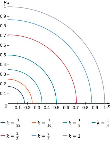
The level curves \(f(x,y)=k\) of the function f are given in the following graph, where k is a constant.
- Apply the midpoint rule with \(m=n=2\) to estimate the double integral \(\underset{R}{∬}f(x,y)dA,\) where \(R=[0.2,1]\,\times \,[0,0.8].\)
- Estimate the average value of the function f on R.
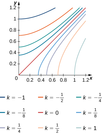
a. \(0.112\) b. \({f}_{\text{ave}}≃0.175;\) here \(f(0.4,0.2)≃0.1,\) \(f(0.2,0.6)≃-0.2,\) \(f(0.8,0.2)≃0.6,\) and \(f(0.8,0.6)≃0.2.\)
The level curves \(f(x,y)=k\) of the function f are given in the following graph, where k is a constant.
- Apply the midpoint rule with \(m=n=2\) to estimate the double integral \(\underset{R}{∬}f(x,y)dA,\) where \(R=[0.1,0.5]\,\times \,[0.1,0.5].\)
- Estimate the average value of the function f on R.
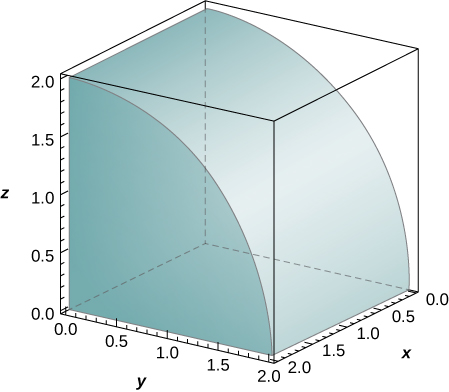
The solid lying under the surface \(z=\sqrt{4-{y}^{2}}\) and above the rectangular region \(R=[0,2]\,\times \,[0,2]\) is illustrated in the following graph. Evaluate the double integral \(\underset{R}{∬}f(x,y)dA,\) where \(f(x,y)=\sqrt{4-{y}^{2}},\) by finding the volume of the corresponding solid.
\(2\pi .\)
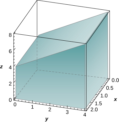
The solid lying under the plane \(z=y+4\) and above the rectangular region \(R=[0,2]\,\times \,[0,4]\) is illustrated in the following graph. Evaluate the double integral \(\underset{R}{∬}f(x,y)dA,\) where \(f(x,y)=y+4,\) by finding the volume of the corresponding solid.
In the following exercises, calculate the integrals by interchanging the order of integration.
\(\int_{-1}^{1}\int_{-2}^{2}(2x+3y+5)dx\,dy\)
40.
\(\int_{0}^{2}\int_{0}^{1}(x+2{e}^{y}-3)dx\,dy\)
\(\int_{1}^{27}\int_{1}^{2}(\sqrt[3]{x}+\sqrt[3]{y})dy\,dx\)
\(\frac{81}{2}+39\sqrt[3]{2}.\)
\(\int_{1}^{16}\int_{1}^{8}(\sqrt[4]{x}+2\sqrt[3]{y})dy\,dx\)
\(\int_{\text{ln}\,2}^{\text{ln}\,3}\int_{0}^{1}{e}^{x+y}dy\,dx\)
\(e-1.\)
\(\int_{0}^{2}\int_{0}^{1}{3}^{x+y}dy\,dx\)
\(\int_{1}^{6}\int_{2}^{9}\frac{\sqrt{y}}{{x}^{2}}dy\,dx\)
\(15-\frac{10\sqrt{2}}{9}.\)
\(\int_{1}^{9}\int_{4}^{2}\frac{\sqrt{x}}{{y}^{2}}dy\,dx\)
In the following exercises, evaluate the iterated integrals by choosing the order of integration.
\(\int_{0}^{\pi}\,\int_{0}^{\pi \text{/}2}\text{sin}(2x)\text{cos}(3y)dx\,dy\)
0.
\(\int_{\pi \text{/}12}^{\pi \text{/}8}\,\int_{\pi \text{/}4}^{\pi \text{/}3}[\text{cot}\,x+\text{tan}(2y)]dx\,dy\)
\(\int_{1}^{e}\,\int_{1}^{e}[\frac{1}{x}\text{sin}(\text{ln}\,x)+\frac{1}{y}\text{cos}(\text{ln}\,y)]dx\,dy\)
\((e-1)(1+\text{sin}\,1-\text{cos}\,1).\)
\(\int_{1}^{e}\,\int_{1}^{e}\frac{\text{sin}(\text{ln}\,x)\text{cos}(\text{ln}\,y)}{xy}dx\,dy\)
\(\int_{1}^{2}\,\int_{1}^{2}(\frac{\text{ln}\,y}{x}+\frac{x}{2y+1})dy\,dx\)
\(\frac{3}{4}\text{ln}(\frac{5}{3})+2\,{\text{ln}}^{2}2-\text{ln}\,2.\)
\(\int_{1}^{e}\,\int_{1}^{2}{x}^{2}\text{ln}(x)dy\,dx\)
\(\int_{1}^{\sqrt{3}}\,\int_{1}^{2}y\,\text{arctan}(\frac{1}{x})dy\,dx\)
\(\frac{1}{8}[(2\sqrt{3}-3)\pi +6\,\text{ln}\,2].\)
\(\int_{0}^{1}\,\int_{0}^{1\text{/}2}(\text{arcsin}\,x+\text{arcsin}\,y)dy\,dx\)
\(\int_{0}^{1}\,\int_{1}^{2}x{e}^{x+4y}dy\,dx\)
\(\frac{1}{4}{e}^{4}({e}^{4}-1).\)
\(\int_{1}^{2}\,\int_{0}^{1}x{e}^{x-y}dy\,dx\)
\(\int_{1}^{e}\,\int_{1}^{e}(\frac{\text{ln}\,y}{\sqrt{y}}+\frac{\text{ln}\,x}{\sqrt{x}})dy\,dx\)
\(4(e-1)(2-\sqrt{e}).\)
\(\int_{1}^{e}\,\int_{1}^{e}(\frac{x\,\text{ln}\,y}{\sqrt{y}}+\frac{y\,\text{ln}\,x}{\sqrt{x}})dy\,dx\)
\(\int_{0}^{1}\,\int_{1}^{2}(\frac{x}{{x}^{2}+{y}^{2}})dy\,dx\)
\(-\frac{\pi }{4}+\text{ln}(\frac{5}{4})-\frac{1}{2}\text{ln}\,2+\text{arctan}\,2.\)
\(\int_{0}^{1}\,\int_{1}^{2}\frac{y}{x+{y}^{2}}dy\,dx\)
In the following exercises, find the average value of the function over the given rectangles.
\(f(x,y)=\text{-}x+2y,\) \(R=[0,1]\,\times \,[0,1]\)
\(\frac{1}{2}.\)
\(f(x,y)={x}^{4}+2{y}^{3},\) \(R=[1,2]\,\times \,[2,3]\)
\(f(x,y)=\text{sinh}\,x+\text{sinh}\,y,\) \(R=[0,1]\,\times \,[0,2]\)
\(\frac{1}{2}\left(2\,\text{cosh}\,1+\text{cosh}\,2-3\right).\)
\(f(x,y)=\text{arctan}(xy),\) \(R=[0,1]\,\times \,[0,1]\)
Let f and g be two continuous functions such that \(0\le {m}_{1}\le f(x)\le {M}_{1}\) for any \(x\in [a,b]\) and \(0\le {m}_{2}\le g(y)\le {M}_{2}\) for any \(y\in [c,d].\) Show that the following inequality is true:
\({m}_{1}{m}_{2}(b-a)(d-c)\le \int_{a}^{b}\,\int_{c}^{d}f(x)g(y)dy\,dx\le {M}_{1}{M}_{2}(b-a)(d-c).\)
In the following exercises, use property v. of double integrals and the answer from the preceding exercise to show that the following inequalities are true.
\(\frac{1}{{e}^{2}}\le \underset{R}{∬}{e}^{\text{-}{x}^{2}-{y}^{2}}dA\le 1,\) where \(R=[0,1]\,\times \,[0,1]\)
\(\frac{{\pi }^{2}}{144}\le \underset{R}{∬}\text{sin}\,x\,\text{cos}\,y\,dA\le \frac{{\pi }^{2}}{48},\) where \(R=[\frac{\pi }{6},\frac{\pi }{3}]\,\times \,[\frac{\pi }{6},\frac{\pi }{3}]\)
\(0\le \underset{R}{∬}{e}^{\text{-}y}\text{cos}\,x\,dA\le {\left(\frac{\pi }{2}\right)}^{2},\) where \(R=[0,\frac{\pi }{2}]\,\times \,[0,\frac{\pi }{2}]\)
\(0\le \underset{R}{∬}(\text{ln}\,x)(\text{ln}\,y)dA\le {(e-1)}^{2},\) where \(R=[1,e]\,\times \,[1,e]\)
Let f and g be two continuous functions such that \(0\le {m}_{1}\le f(x)\le {M}_{1}\) for any \(x\in [a,b]\) and \(0\le {m}_{2}\le g(y)\le {M}_{2}\) for any \(y\in [c,d].\) Show that the following inequality is true:
\(({m}_{1}+{m}_{2})(b-a)(d-c)\le \int_{a}^{b}\,\int_{c}^{d}[f(x)+g(y)]dy\,dx\le ({M}_{1}+{M}_{2})(b-a)(d-c).\)
In the following exercises, use property v. of double integrals and the answer from the preceding exercise to show that the following inequalities are true.
\(\frac{2}{e}\le \underset{R}{∬}({e}^{\text{-}{x}^{2}}+{e}^{\text{-}{y}^{2}})dA\le 2,\) where \(R=[0,1]\,\times \,[0,1]\)
\(\frac{{\pi }^{2}}{36}\le \underset{R}{∬}(\text{sin}\,x+\text{cos}\,y)dA\le \frac{{\pi }^{2}\sqrt{3}}{36},\) where \(R=[\frac{\pi }{6},\frac{\pi }{3}]\,\times \,[\frac{\pi }{6},\frac{\pi }{3}]\)
\(\frac{{\pi }^{2}}{4}{e}^{\frac{-\pi }{2}}\le \underset{R}{∬}(\text{cos}\,x+{e}^{-y})dA\le \frac{{\pi }^{2}}{2},\) where \(R=[0,\frac{\pi }{2}]\,\times \,[0,\frac{\pi }{2}]\)
\(0\le \underset{R}{∬}(\text{ln} x+\text{ln}\,y)dA\le 2{\left(e-1\right)}^{2},\) where \(R=[1,e]\,\times \,[1,e]\)
In the following exercises, the function f is given in terms of double integrals.
- Determine the explicit form of the function f.
- Find the volume of the solid under the surface \(z=f(x,y)\) and above the region R.
- Find the average value of the function f on R.
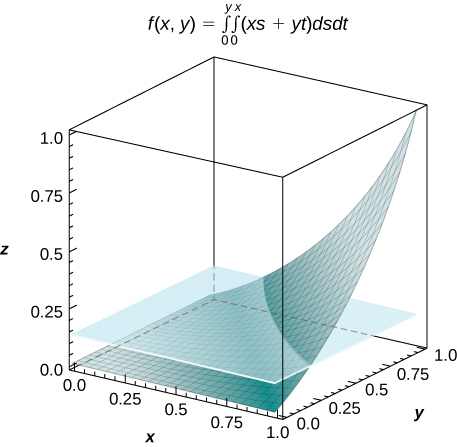
- Use a computer algebra system (CAS) to plot \(z=f(x,y)\) and \(z={f}_{\text{ave}}\) in the same system of coordinates.
[T] \(f(x,y)=\int_{0}^{y}\,\int_{0}^{x}(xs+yt)ds\,dt,\) where \((x,y)\in R=[0,1]\,\times \,[0,1]\)
a. \(f(x,y)=\frac{1}{2}xy({x}^{2}+{y}^{2})\) b. \(V=\int_{0}^{1}\,\int_{0}^{1}f(x,y)dx\,dy=\frac{1}{8}\) c. \({f}_{\text{ave}}=\frac{1}{8};\)
d.
[T] \(f(x,y)=\int_{0}^{x}\,\int_{0}^{y}[\text{cos}(s)+\text{cos}(t)]dt\,ds,\) where \((x,y)\in R=[0,3]\,\times \,[0,3]\)
Show that if f and g are continuous on \([a,b]\) and \([c,d],\) respectively, then
\(\int_{a}^{b}\,\int_{c}^{d}[f(x)+g(y)]dy\,dx=(d-c)\int_{a}^{b}f(x)dx\)
\(\,+\int_{a}^{b}\,\int_{c}^{d}g(y)dy\,dx=(b-a)\int_{c}^{d}g(y)dy+\int_{c}^{d}\,\int_{a}^{b}f(x)dx\,dy.\)
Show that \(\int_{a}^{b}\,\int_{c}^{d}yf(x)+xg(y)dy\,dx=\frac{1}{2}({d}^{2}-{c}^{2})(\int_{a}^{b}f(x)dx)+\frac{1}{2}({b}^{2}-{a}^{2})(\int_{c}^{d}g(y)dy).\)
[T] Consider the function \(f(x,y)={e}^{\text{-}{x}^{2}-{y}^{2}},\) where \((x,y)\in R=[-1,1]\,\times \,[-1,1].\)
- Use the midpoint rule with \(m=n=2,4\text{,…,}\,10\) to estimate the double integral \(I=\underset{R}{∬}{e}^{\text{-}{x}^{2}-{y}^{2}}dA.\) Round your answers to the nearest hundredths.
- For \(m=n=2,\) find the average value of f over the region R. Round your answer to the nearest hundredths.
- Use a CAS to graph in the same coordinate system the solid whose volume is given by \(\underset{R}{∬}{e}^{\text{-}{x}^{2}-{y}^{2}}dA\) and the plane \(z={f}_{\text{ave}}.\)
a. For \(m=n=2,\) \(I=4{e}^{-0.5}\approx 2.43\) b. \({f}_{\text{ave}}={e}^{-0.5}≃0.61;\)
c.
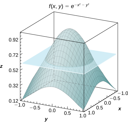
[T] Consider the function \(f(x,y)=\text{sin}({x}^{2})\text{cos}({y}^{2}),\) where \((x,y)\in R=[-1,1]\,\times \,[-1,1].\)
- Use the midpoint rule with \(m=n=2,4\text{,…,}\,10\) to estimate the double integral \(I=\underset{R}{∬}\text{sin}({x}^{2})\text{cos}({y}^{2})dA.\) Round your answers to the nearest hundredths.
- For \(m=n=2,\) find the average value of f over the region R. Round your answer to the nearest hundredths.
- Use a CAS to graph in the same coordinate system the solid whose volume is given by \(\underset{R}{∬}\text{sin}({x}^{2})\text{cos}({y}^{2})dA\) and the plane \(z={f}_{\text{ave}}.\)
In the following exercises, the functions \({f}_{n}\) are given, where \(n\ge 1\) is a natural number.
- Find the volume of the solids \({S}_{n}\) under the surfaces \(z={f}_{n}(x,y)\) and above the region R.
- Determine the limit of the volumes of the solids \({S}_{n}\) as n increases without bound.
\({f}_{n}(x,y)={x}^{n}+{y}^{n}+xy,(x,y)\in R=[0,1]\,\times \,[0,1]\)
a. \(\frac{2}{n+1}+\frac{1}{4}\) b. \(\frac{1}{4}\)
\({f}_{n}(x,y)=\frac{1}{{x}^{n}}+\frac{1}{{y}^{n}},(x,y)\in R=[1,2]\,\times \,[1,2]\)
Show that the average value of a function f on a rectangular region \(R=[a,b]\,\times \,[c,d]\) is \({f}_{\text{ave}}\approx \frac{1}{mn}\sum_{i=1}^{m}\sum_{j=1}^{n}f({x}_{ij}^{*},{y}_{ij}^{*}),\) where \(({x}_{ij}^{*},{y}_{ij}^{*})\) are the sample points of the partition of R, where \(1\le i\le m\) and \(1\le j\le n.\)
Use the midpoint rule with \(m=n\) to show that the average value of a function f on a rectangular region \(R=[a,b]\,\times \,[c,d]\) is approximated by
\[{f}_{\text{ave}}\approx \frac{1}{{n}^{2}}\sum_{i,j=1}^{n}f(\frac{1}{2}({x}_{i-1}+{x}_{i}),\frac{1}{2}({y}_{j-1}+{y}_{j})).\]
An isotherm map is a chart connecting points having the same temperature at a given time for a given period of time. Use the preceding exercise and apply the midpoint rule with \(m=n=2\) to find the average temperature over the region given in the following figure.
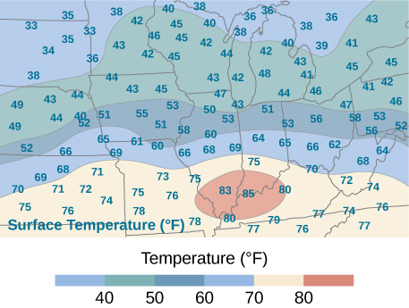
\(56.5\text{°}\) F; here \(f({x}_{1}^{*},{y}_{1}^{*})=71,\) \(f({x}_{2}^{*},{y}_{1}^{*})=72,\) \(f({x}_{1}^{*},{y}_{2}^{*})=40,\) \(f({x}_{2}^{*},{y}_{2}^{*})=43,\) where \({x}_{i}^{*}\) and \({y}_{j}^{*}\) are the midpoints of the subintervals of the partitions of \([a,b]\) and \([c,d],\) respectively.
Glossary
- double integral
- of the function \(f(x,y)\) over the region \(R\) in the \(xy\) -plane is defined as the limit of a double Riemann sum, \(\underset{R}{∬}f(x,y)dA=\underset{m,n\to \infty }{\text{lim}}\sum_{i=1}^{m}\sum_{j=1}^{n}f({x}_{ij}^{*},{y}_{ij}^{*})\Delta A.\)
- double Riemann sum
- of the function \(f(x,y)\) over a rectangular region \(R\) is \(\sum_{i=1}^{m}\sum_{j=1}^{n}f({x}_{ij}^{*},{y}_{ij}^{*})\Delta A\) where \(R\) is divided into smaller subrectangles \({R}_{ij}\) and \(({x}_{ij}^{*},{y}_{ij}^{*})\) is an arbitrary point in \({R}_{ij}\)
- Fubini’s theorem
- if \(f(x,y)\) is a function of two variables that is continuous over a rectangular region \(R=\left\{(x,y)\in {ℝ}^{2}|a\le x\le b,c\le y\le d\},\right.\) then the double integral of \(f\) over the region equals an iterated integral, \(\underset{R}{∬}f(x,y)dy\,dx={∫}_{a}^{b}{∫}_{c}^{d}f(x,y)dx\,dy={∫}_{c}^{d}{∫}_{a}^{b}f(x,y)dx\,dy\)
- iterated integral
- for a function \(f(x,y)\) over the region \(R\) is where \(a,b,c,\) and \(d\) are any real numbers and \(R=[a,b]\,\times \,[c,d]\)