Section 1.3Polar Coordinates
The rectangular coordinate system (or Cartesian plane) provides a means of mapping points to ordered pairs and ordered pairs to points. This is called a one-to-one mapping from points in the plane to ordered pairs. The polar coordinate system provides an alternative method of mapping points to ordered pairs. In this section we see that in some circumstances, polar coordinates can be more useful than rectangular coordinates.
Defining Polar Coordinates
To find the coordinates of a point in the polar coordinate system, consider Figure 1. The point \(P\) has Cartesian coordinates \((x,y).\) The line segment connecting the origin to the point \(P\) measures the distance from the origin to \(P\) and has length \(r.\) The angle between the positive \(x\) -axis and the line segment has measure \(θ.\) This observation suggests a natural correspondence between the coordinate pair \((x,y)\) and the values \(r\) and \(θ.\) This correspondence is the basis of the polar coordinate system. Note that every point in the Cartesian plane has two values (hence the term ordered pair) associated with it. In the polar coordinate system, each point also has two values associated with it: \(r\) and \(θ.\)
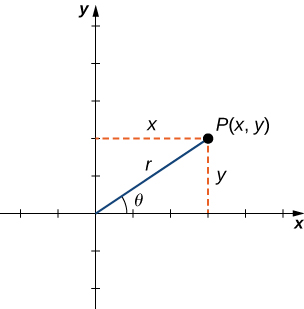
Using right-triangle trigonometry, the following equations are true for the point \(P\text{:}\)
\[\text{cos}\,θ=\frac{x}{r}\,\text{so}\,x=r\,\text{cos}\,θ\]
\[\text{sin}\,θ=\frac{y}{r}\,\text{so}\,y=r\,\text{sin}\,θ.\]
Furthermore,
\[{r}^{2}={x}^{2}+{y}^{2}\,\text{and}\,\text{tan}\,θ=\frac{y}{x}.\]
Each point \((x,y)\) in the Cartesian coordinate system can therefore be represented as an ordered pair \((r,θ)\) in the polar coordinate system. The first coordinate is called the radial coordinate and the second coordinate is called the angular coordinate. Every point in the plane can be represented in this form.
Note that the equation \(\text{tan}\,θ=y\text{/}x\) has an infinite number of solutions for any ordered pair \((x,y).\) However, if we restrict the solutions to values between \(0\) and \(2\pi\) then we can assign a unique solution to the quadrant in which the original point \((x,y)\) is located. Then the corresponding value of r is positive, so \({r}^{2}={x}^{2}+{y}^{2}.\)
Given a point \(P\) in the plane with Cartesian coordinates \((x,y)\) and polar coordinates \((r,θ),\) the following conversion formulas hold true:
\[x=r\,\text{cos}\,θ\,\text{and}\,y=r\,\text{sin}\,θ,\]
\[{r}^{2}={x}^{2}+{y}^{2}\,\text{and}\,\text{tan}\,θ=\frac{y}{x}.\]
These formulas can be used to convert from rectangular to polar or from polar to rectangular coordinates.
Convert each of the following points into polar coordinates.
- \((1,1)\)
- \((-3,4)\)
- \((0,3)\)
- \((5\sqrt{3},-5)\)
Convert each of the following points into rectangular coordinates.
- \((3,\pi \text{/}3)\)
- \((2,3\pi \text{/}2)\)
- \((6,-5\pi \text{/}6)\)
For each rectangular point use \({r}^{2}={x}^{2}+{y}^{2}\) and \(\text{tan}\,θ=y\text{/}x;\) for each polar point use \(x=r\,\text{cos}\,θ\) and \(y=r\,\text{sin}\,θ.\)
- Use \(x=1\) and \(y=1\) in Equation 5:
Therefore this point can be represented as \((\sqrt{2},\frac{\pi }{4})\) in polar coordinates.\[\begin{array}{lllllll}\begin{array}{lll}{r}^{2} & = & {x}^{2}+{y}^{2} \\ & = & {1}^{2}+{1}^{2} \\ r & = & \sqrt{2}\end{array} & & & \text{and} & & & \begin{array}{lll}\text{tan}\,θ & = & \frac{y}{x} \\ & = & \frac{1}{1}=1 \\ θ & = & \frac{\pi }{4}.\end{array}\end{array}\]
- Use \(x=-3\) and \(y=4\) in Equation 5:
The point \((-3, 4)\) lies in Quadrant \(\text{II}\) . Subtract the value of the reference angle, \(\text{arctan}\left(\frac{4}{3}\right)\) , from \(\pi\) to find the radian measure of \(θ\) .
Therefore this point can be represented as \((5,2.21)\) in polar coordinates.\[\begin{array}{lllllll}\begin{array}{lll}{r}^{2} & = & {x}^{2}+{y}^{2} \\ & = & {(-3)}^{2}+{(4)}^{2} \\ r & = & 5\end{array} & & & \text{and} & & & \begin{array}{lll}\text{tan}\,θ & = & \frac{y}{x} \\ & = & -\frac{4}{3} \\ θ & = & \pi -arctan(\frac{4}{3}) \\ & \approx & 2.21.\end{array}\end{array}\]
- Use \(x=0\) and \(y=3\) in Equation 5:
Direct application of the second equation leads to division by zero. Graphing the point \((0,3)\) on the rectangular coordinate system reveals that the point is located on the positive y-axis. The angle between the positive x-axis and the positive y-axis is \(\frac{\pi }{2}.\) Therefore this point can be represented as \((3,\frac{\pi }{2})\) in polar coordinates.\[\begin{array}{lllllll}\begin{array}{lll}{r}^{2} & = & {x}^{2}+{y}^{2} \\ & = & {(3)}^{2}+{(0)}^{2} \\ & = & 9+0 \\ r & = & 3\end{array} & & & \text{and} & & & \begin{array}{lll}\text{tan}\,θ & = & \frac{y}{x} \\ & = & \frac{3}{0}.\end{array}\end{array}\]
- Use \(x=5\sqrt{3}\) and \(y=-5\) in Equation 5:
Therefore this point can be represented as \((10,-\frac{\pi }{6})\) in polar coordinates.\[\begin{array}{lllllll}\begin{array}{lll}{r}^{2} & = & {x}^{2}+{y}^{2} \\ & = & {(5\sqrt{3})}^{2}+{(-5)}^{2} \\ & = & 75+25 \\ r & = & 10\end{array} & & & \text{and} & & & \begin{array}{lll}\text{tan}\,θ & = & \frac{y}{x} \\ & = & \frac{-5}{5\sqrt{3}}=-\frac{\sqrt{3}}{3} \\ θ & = & -\frac{\pi }{6}.\end{array}\end{array}\]
- Use \(r=3\) and \(θ=\frac{\pi }{3}\) in Equation 4:
Therefore this point can be represented as \((\frac{3}{2},\,\frac{3\sqrt{3}}{2})\) in rectangular coordinates.\[\begin{array}{lllllll}\begin{array}{lll}x & = & r\,\text{cos}\,θ \\ & = & 3\,\text{cos}(\frac{\pi }{3}) \\ & = & 3(\frac{1}{2})=\frac{3}{2}\end{array} & & & \text{and} & & & \begin{array}{lll}y & = & r\,\text{sin}\,θ \\ & = & 3\,\text{sin}(\frac{\pi }{3}) \\ & = & 3(\frac{\sqrt{3}}{2})=\frac{3\sqrt{3}}{2}.\end{array}\end{array}\]
- Use \(r=2\) and \(θ=\frac{3\pi }{2}\) in Equation 4:
Therefore this point can be represented as \((0,-2)\) in rectangular coordinates.\[\begin{array}{lllllll}\begin{array}{lll}x & = & r\,\text{cos}\,θ \\ & = & 2\,\text{cos}(\frac{3\pi }{2}) \\ & = & 2(0)=0\end{array} & & & \text{and} & & & \begin{array}{lll}y & = & r\,\text{sin}\,θ \\ & = & 2\,\text{sin}(\frac{3\pi }{2}) \\ & = & 2(-1)=-2.\end{array}\end{array}\]
- Use \(r=6\) and \(θ=-\frac{5\pi }{6}\) in Equation 4:
Therefore this point can be represented as \((-3\sqrt{3},-3)\) in rectangular coordinates.\[\begin{array}{lllllll}\begin{array}{lll}x & = & r\,\text{cos}\,θ \\ & = & 6\,\text{cos}(-\frac{5\pi }{6}) \\ & = & 6(-\frac{\sqrt{3}}{2}) \\ & = & -3\sqrt{3}\end{array} & & & \text{and} & & & \begin{array}{lll}y & = & r\,\text{sin}\,θ \\ & = & 6\,\text{sin}(-\frac{5\pi }{6}) \\ & = & 6(-\frac{1}{2}) \\ & = & -3.\end{array}\end{array}\]
Convert \((-8,-8)\) into polar coordinates and \((4,\frac{2\pi }{3})\) into rectangular coordinates.
\((8\sqrt{2},\frac{5\pi }{4})\) and \((-2,2\sqrt{3})\)
The polar representation of a point is not unique. For example, the polar coordinates \((2,\frac{\pi }{3})\) and \((2,\frac{7\pi }{3})\) both represent the point \((1,\sqrt{3})\) in the rectangular system. Also, the value of \(r\) can be negative. Therefore, the point with polar coordinates \((-2,\frac{4\pi }{3})\) also represents the point \((1,\sqrt{3})\) in the rectangular system, as we can see by using Equation 5:
\[\begin{array}{lllllll}\begin{array}{lll}x & = & r\,\text{cos}\,θ \\ & = & -2\,\text{cos}(\frac{4\pi }{3}) \\ & = & -2(-\frac{1}{2})=1\end{array} & & & \text{and} & & & \begin{array}{lll}y & = & r\,\text{sin}\,θ \\ & = & -2\,\text{sin}(\frac{4\pi }{3}) \\ & = & -2(-\frac{\sqrt{3}}{2})=\sqrt{3}.\end{array}\end{array}\]
Every point in the plane has an infinite number of representations in polar coordinates. However, each point in the plane has only one representation in the rectangular coordinate system.
Note that the polar representation of a point in the plane also has a visual interpretation. In particular, \(r\) is the directed distance that the point lies from the origin, and \(θ\) measures the angle that the line segment from the origin to the point makes with the positive \(x\) -axis. Positive angles are measured in a counterclockwise direction and negative angles are measured in a clockwise direction. The polar coordinate system appears in the following figure.
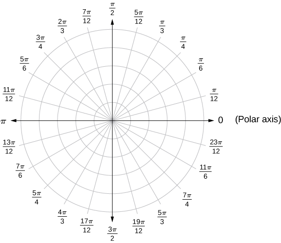
The line segment starting from the center of the graph going to the right (called the positive x-axis in the Cartesian system) is the polar axis. The center point is the pole, or origin, of the coordinate system, and corresponds to \(r=0.\) The innermost circle shown in Figure 2 contains all points a distance of 1 unit from the pole, and is represented by the equation \(r=1.\) Then \(r=2\) is the set of points 2 units from the pole, and so on. The line segments emanating from the pole correspond to fixed angles. To plot a point in the polar coordinate system, start with the angle. If the angle is positive, then measure the angle from the polar axis in a counterclockwise direction. If it is negative, then measure it clockwise. If the value of \(r\) is positive, move that distance along the terminal ray of the angle. If it is negative, move along the ray that is opposite the terminal ray of the given angle.
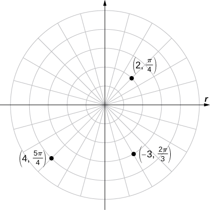
Plot each of the following points on the polar plane.
- \((2,\frac{\pi }{4})\)
- \((-3,\frac{2\pi }{3})\)
- \((4,\frac{5\pi }{4})\)
Start with the angle θ, measured from the polar axis, then move out along that ray by r (or along the opposite ray if r is negative).
The three points are plotted in the following figure.
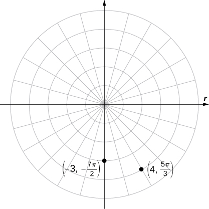
Plot \((4,\frac{5\pi }{3})\) and \((-3,-\frac{7\pi }{2})\) on the polar plane.
Polar Curves
Now that we know how to plot points in the polar coordinate system, we can discuss how to plot curves. In the rectangular coordinate system, we can graph a function \(y=f(x)\) and create a curve in the Cartesian plane. In a similar fashion, we can graph a curve that is generated by a function \(r=f(θ).\)
The general idea behind graphing a function in polar coordinates is the same as graphing a function in rectangular coordinates. Start with a list of values for the independent variable \((θ\) in this case) and calculate the corresponding values of the dependent variable \(r.\) This process generates a list of ordered pairs, which can be plotted in the polar coordinate system. Finally, connect the points, and take advantage of any patterns that may appear. The function may be periodic, for example, which indicates that only a limited number of values for the independent variable are needed.
- Create a table with two columns. The first column is for \(θ,\) and the second column is for \(r.\)
- Create a list of values for \(θ.\)
- Calculate the corresponding \(r\) values for each \(θ.\)
- Plot each ordered pair \((r,θ)\) on the coordinate axes.
- Connect the points and look for a pattern.
Watch this video for more information on sketching polar curves.
Graph the curve defined by the function \(r=4\,\text{sin}\,θ.\) Identify the curve and rewrite the equation in rectangular coordinates.
Build a table of \((θ,r)\) values over one period and plot the points; to convert, multiply both sides by r so you can substitute \({r}^{2}={x}^{2}+{y}^{2}\) and \(y=r\,\text{sin}\,θ.\)
Because the function is a multiple of a sine function, it is periodic with period \(2\pi ,\) so use values for \(θ\) between 0 and \(2\pi .\) The result of steps 1–3 appear in the following table. Figure 4 shows the graph based on this table.
| \(θ\) | \(r=4\,\text{sin}\,θ\) | \(θ\) | \(r=4\,\text{sin}\,θ\) | |
| 0 | 0 | \(\pi\) | 0 | |
| \(\frac{\pi }{6}\) | \(2\) | \(\frac{7\pi }{6}\) | \(-2\) | |
| \(\frac{\pi }{4}\) | \(2\sqrt{2}\approx 2.8\) | \(\frac{5\pi }{4}\) | \(-2\sqrt{2}\approx -2.8\) | |
| \(\frac{\pi }{3}\) | \(2\sqrt{3}\approx 3.4\) | \(\frac{4\pi }{3}\) | \(-2\sqrt{3}\approx -3.4\) | |
| \(\frac{\pi }{2}\) | \(4\) | \(\frac{3\pi }{2}\) | \(-4\) | |
| \(\frac{2\pi }{3}\) | \(2\sqrt{3}\approx 3.4\) | \(\frac{5\pi }{3}\) | \(-2\sqrt{3}\approx -3.4\) | |
| \(\frac{3\pi }{4}\) | \(2\sqrt{2}\approx 2.8\) | \(\frac{7\pi }{4}\) | \(-2\sqrt{2}\approx -2.8\) | |
| \(\frac{5\pi }{6}\) | \(2\) | \(\frac{11\pi }{6}\) | \(-2\) | |
| \(2\pi\) | 0 |
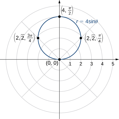
This is the graph of a circle. The equation \(r=4\,\text{sin}\,θ\) can be converted into rectangular coordinates by first multiplying both sides by \(r.\) This gives the equation \({r}^{2}=4r\,\text{sin}\,θ.\) Next use the facts that \({r}^{2}={x}^{2}+{y}^{2}\) and \(y=r\,\text{sin}\,θ.\) This gives \({x}^{2}+{y}^{2}=4y.\) To put this equation into standard form, subtract \(4y\) from both sides of the equation and complete the square:
\[\begin{array}{lll}{x}^{2}+{y}^{2}-4y & = & 0 \\ {x}^{2}+({y}^{2}-4y) & = & 0 \\ {x}^{2}+({y}^{2}-4y+4) & = & 0+4 \\ {x}^{2}+{(y-2)}^{2} & = & 4.\end{array}\]
This is the equation of a circle with radius 2 and center \((0,2)\) in the rectangular coordinate system.
Create a graph of the curve defined by the function \(r=4+4\,\text{cos}\,θ.\)
The name of this shape is a cardioid, which we will study further later in this section.
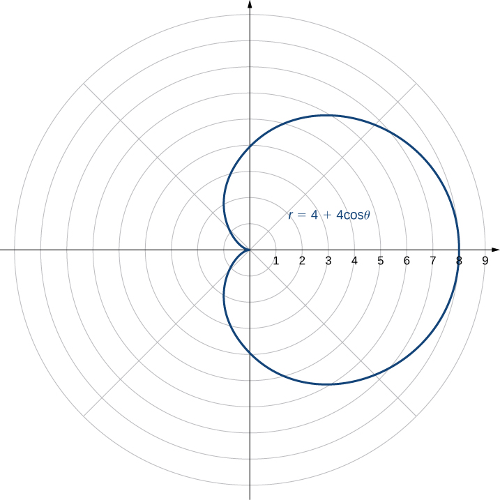
The graph in Example 3 was that of a circle. The equation of the circle can be transformed into rectangular coordinates using the coordinate transformation formulas in Equation 5. Example 5 gives some more examples of functions for transforming from polar to rectangular coordinates.
Rewrite each of the following equations in rectangular coordinates and identify the graph.
- \(θ=\frac{\pi }{3}\)
- \(r=3\)
- \(r=6\,\text{cos}\,θ-8\,\text{sin}\,θ\)
Multiply by r where needed so you can substitute \({r}^{2}={x}^{2}+{y}^{2},\,x=r\,\text{cos}\,θ,\) and \(y=r\,\text{sin}\,θ,\) then complete the square if the result isn't already in standard form.
- Take the tangent of both sides. This gives \(\text{tan}\,θ=\text{tan}(\pi \text{/}3)=\sqrt{3}.\) Since \(\text{tan}\,θ=y\text{/}x\) we can replace the left-hand side of this equation by \(y\text{/}x.\) This gives \(y\text{/}x=\sqrt{3},\) which can be rewritten as \(y=x\sqrt{3}.\) This is the equation of a straight line passing through the origin with slope \(\sqrt{3}.\) In general, any polar equation of the form \(θ=K\) represents a straight line through the pole with slope equal to \(\text{tan}\,K.\)
- First, square both sides of the equation. This gives \({r}^{2}=9.\) Next replace \({r}^{2}\) with \({x}^{2}+{y}^{2}.\) This gives the equation \({x}^{2}+{y}^{2}=9,\) which is the equation of a circle centered at the origin with radius 3. In general, any polar equation of the form \(r=k\) where k is a positive constant represents a circle of radius k centered at the origin. (Note: when squaring both sides of an equation it is possible to introduce new points unintentionally. This should always be taken into consideration. However, in this case we do not introduce new points. For example, \((-3,\frac{\pi }{3})\) is the same point as \((3,\frac{4\pi }{3}).)\)
- Multiply both sides of the equation by \(r.\) This leads to \({r}^{2}=6r\,\text{cos}\,θ-8r\,\text{sin}\,θ.\) Next use the formulas
This gives
To put this equation into standard form, first move the variables from the right-hand side of the equation to the left-hand side, then complete the square.
This is the equation of a circle with center at \((3,-4)\) and radius 5. Notice that the circle passes through the origin since the center is 5 units away.\[{r}^{2}={x}^{2}+{y}^{2},\,x=r\,\text{cos}\,θ,\,y=r\,\text{sin}\,θ.\]
\[\begin{array}{lll}{r}^{2} & = & 6(r\,\text{cos}\,θ)-8(r\,\text{sin}\,θ) \\ {x}^{2}+{y}^{2} & = & 6x-8y.\end{array}\]
\[\begin{array}{lll}{x}^{2}+{y}^{2} & = & 6x-8y \\ {x}^{2}-6x+{y}^{2}+8y & = & 0 \\ ({x}^{2}-6x)+({y}^{2}+8y) & = & 0 \\ ({x}^{2}-6x+9)+({y}^{2}+8y+16) & = & 9+16 \\ {(x-3)}^{2}+{(y+4)}^{2} & = & 25.\end{array}\]
Rewrite the equation \(r=\text{sec}\,θ\,\text{tan}\,θ\) in rectangular coordinates and identify its graph.
\(y={x}^{2},\) which is the equation of a parabola opening upward.
We have now seen several examples of drawing graphs of curves defined by polar equations. A summary of some common curves is given in the tables below. In each equation, a and b are arbitrary constants.
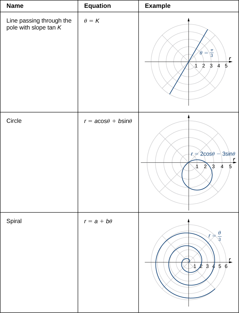
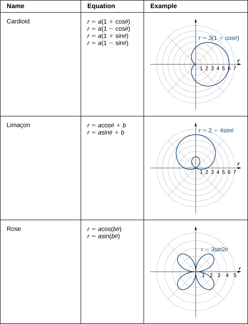
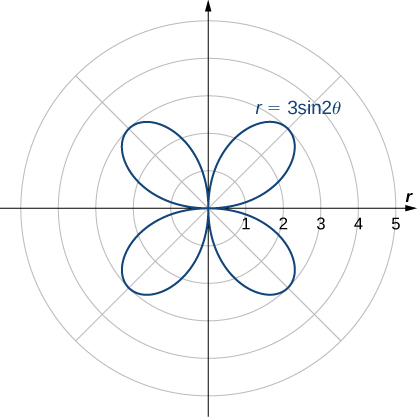
A cardioid is a special case of a limaçon (pronounced “lee-mah-son”), in which \(a=b\) or \(a=\text{-}b.\) The rose is a very interesting curve. Notice that the graph of \(r=3\,\text{sin}\,2θ\) has four petals. However, the graph of \(r=3\,\text{sin}\,3θ\) has three petals as shown.
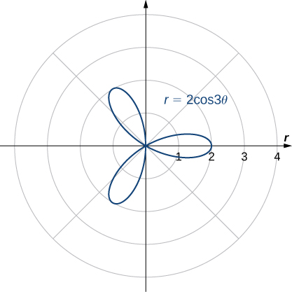
If the coefficient of \(θ\) is even, the graph has twice as many petals as the coefficient. If the coefficient of \(θ\) is odd, then the number of petals equals the coefficient. You are encouraged to explore why this happens — try it in Figure 7 above. Even more interesting graphs emerge when the coefficient of \(θ\) is not an integer. For example, if it is rational, then the curve is closed; that is, it eventually ends where it started (try \(k=2.5\)). However, if the coefficient is irrational, then the curve never closes (try \(k=3.14159,\) close to \(π\)). Although it may appear that the curve is closed, a closer examination reveals that the petals just above the positive r axis are slightly thicker. This is because the petal does not quite match up with the starting point.
Recall the chambered nautilus introduced in the chapter opener. This creature displays a spiral when half the outer shell is cut away. It is possible to describe a spiral using rectangular coordinates. Figure 8 shows a spiral in rectangular coordinates. How can we describe this curve mathematically?
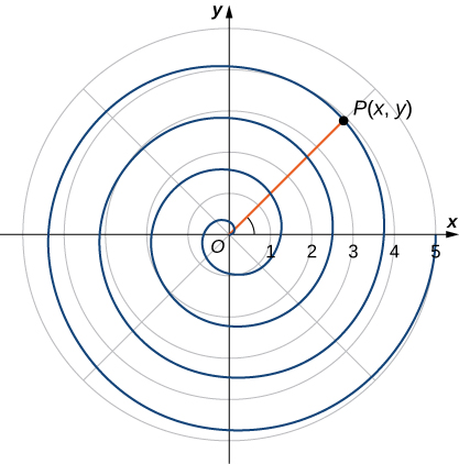
Let the distance from the origin be a constant multiple k of θ, so \(d(P,O)=kθ,\) then rewrite that relationship using \(r=d(P,O).\)
As the point P travels around the spiral in a counterclockwise direction, its distance d from the origin increases. Assume that the distance d is a constant multiple k of the angle \(θ\) that the line segment OP makes with the positive r-axis. Therefore \(d(P,O)=kθ,\) where \(O\) is the origin. Now use the distance formula and some trigonometry:
\[\begin{array}{lll}d(P,O) & = & kθ \\ \sqrt{{(x-0)}^{2}+{(y-0)}^{2}} & = & k\,\text{arctan}(\frac{y}{x}) \\ \sqrt{{x}^{2}+{y}^{2}} & = & k\,\text{arctan}(\frac{y}{x}) \\ \text{arctan}(\frac{y}{x}) & = & \frac{\sqrt{{x}^{2}+{y}^{2}}}{k} \\ y & = & x\,\text{tan}(\frac{\sqrt{{x}^{2}+{y}^{2}}}{k}).\end{array}\]
Although this equation describes the spiral, it is not possible to solve it directly for either x or y. However, if we use polar coordinates, the equation becomes much simpler. In particular, \(d(P,O)=r,\) and \(θ\) is the second coordinate. Therefore the equation for the spiral becomes \(r=kθ.\) Note that when \(θ=0\) we also have \(r=0,\) so the spiral emanates from the origin. We can remove this restriction by adding a constant to the equation. Then the equation for the spiral becomes \(r=a+kθ\) for arbitrary constants \(a\) and \(k.\) This is referred to as an Archimedean spiral, after the Greek mathematician Archimedes.
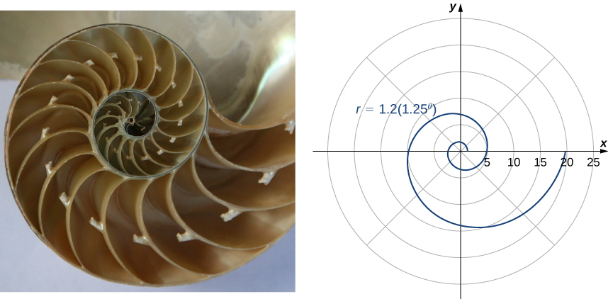
Another type of spiral is the logarithmic spiral, described by the function \(r=a·{b}^{θ}.\) A graph of the function \(r=1.2({1.25}^{θ})\) is given in Figure 9. This spiral describes the shell shape of the chambered nautilus.
Suppose a curve is described in the polar coordinate system via the function \(r=f(θ).\) Since we have conversion formulas from polar to rectangular coordinates given by
\[\begin{array}{l}x=r\,\text{cos}\,θ \\ y=r\,\text{sin}\,θ,\end{array}\]
it is possible to rewrite these formulas using the function
\[\begin{array}{l}x=f(θ)\,\text{cos}\,θ \\ y=f(θ)\,\text{sin}\,θ.\end{array}\]
This step gives a parameterization of the curve in rectangular coordinates using \(θ\) as the parameter. For example, the spiral formula \(r=a+bθ\) from Figure 5 becomes
\[\begin{array}{l}x=(a+bθ)\,\text{cos}\,θ \\ y=(a+bθ)\,\text{sin}\,θ.\end{array}\]
Letting \(θ\) range from \(\text{-}\infty\) to \(\infty\) generates the entire spiral.
Symmetry in Polar Coordinates
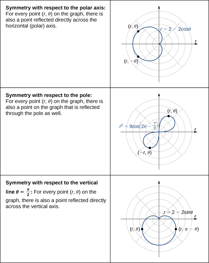
When studying symmetry of functions in rectangular coordinates (i.e., in the form \(y=f(x)),\) we talk about symmetry with respect to the y-axis and symmetry with respect to the origin. In particular, if \(f(\text{-}x)=f(x)\) for all \(x\) in the domain of \(f,\) then \(f\) is an even function and its graph is symmetric with respect to the y-axis. If \(f(\text{-}x)=\text{-}f(x)\) for all \(x\) in the domain of \(f,\) then \(f\) is an odd function and its graph is symmetric with respect to the origin. By determining which types of symmetry a graph exhibits, we can learn more about the shape and appearance of the graph. Symmetry can also reveal other properties of the function that generates the graph. Symmetry in polar curves works in a similar fashion.
Consider a curve generated by the function \(r=f(θ)\) in polar coordinates.
- The curve is symmetric about the polar axis if for every point \((r,θ)\) on the graph, the point \((r,\text{-}θ)\) is also on the graph. Similarly, the equation \(r=f(θ)\) is unchanged by replacing \(θ\) with \(\text{-}θ.\)
- The curve is symmetric about the pole if for every point \((r,θ)\) on the graph, the point \((r,\pi +θ)\) is also on the graph. Similarly, the equation \(r=f(θ)\) is unchanged when replacing \(r\) with \(\text{-}r,\) or \(θ\) with \(\pi +θ.\)
- The curve is symmetric about the vertical line \(θ=\frac{\pi }{2}\) if for every point \((r,θ)\) on the graph, the point \((r,\pi -θ)\) is also on the graph. Similarly, the equation \(r=f(θ)\) is unchanged when \(θ\) is replaced by \(\pi -θ.\)
The following table shows examples of each type of symmetry.
Find the symmetry of the rose defined by the equation \(r=3\,\text{sin}(2θ)\) and create a graph.
Test each symmetry rule in turn by substitution — try \(θ\to \text{-}θ\) first, and if that fails, try \(r\to \text{-}r,\,θ\to \pi -θ\) and see whether either recovers the original equation.
Suppose the point \((r,θ)\) is on the graph of \(r=3\,\text{sin}(2θ).\)
- To test for symmetry about the polar axis, first try replacing \(θ\) with \(\text{-}θ.\) This gives \(r=3\,\text{sin}(2(\text{-}θ))=-3\,\text{sin}(2θ).\) Since this changes the original equation, this test is not satisfied. However, returning to the original equation and replacing \(r\) with \(\text{-}r\) and \(θ\) with \(\pi -θ\) yields
Multiplying both sides of this equation by \(-1\) gives \(r=3\,\text{sin}\,2θ,\) which is the original equation. This demonstrates that the graph is symmetric with respect to the polar axis.\[\begin{array}{l} \\ \text{-}r=3\,\text{sin}(2(\pi -θ)) \\ \text{-}r=3\,\text{sin}(2\pi -2θ) \\ \text{-}r=3\,\text{sin}(-2θ) \\ \text{-}r=-3\,\text{sin}\,2θ.\end{array}\]
- To test for symmetry with respect to the pole, first replace \(r\) with \(\text{-}r,\) which yields \(\text{-}r=3\,\text{sin}(2θ).\) Multiplying both sides by −1 gives \(r=-3\,\text{sin}(2θ),\) which does not agree with the original equation. Therefore the equation does not pass the test for this symmetry. However, returning to the original equation and replacing \(θ\) with \(θ+\pi\) gives
Since this agrees with the original equation, the graph is symmetric about the pole.\[\begin{array}{ll}r & =3\,\text{sin}(2(θ+\pi )) \\ & =3\,\text{sin}(2θ+2\pi ) \\ & =3(\text{sin}\,2θ\,\text{cos}\,2\pi +\text{cos}\,2θ\,\text{sin}\,2\pi ) \\ & =3\,\text{sin}\,2θ.\end{array}\]
- To test for symmetry with respect to the vertical line \(θ=\frac{\pi }{2},\) first replace both \(r\) with \(\text{-}r\) and \(θ\) with \(\text{-}θ.\)
Multiplying both sides of this equation by \(-1\) gives \(r=3\,\text{sin}\,2θ,\) which is the original equation. Therefore the graph is symmetric about the vertical line \(θ=\frac{\pi }{2}.\)\[\begin{array}{l} \\ \text{-}r=3\,\text{sin}(2(\text{-}θ)) \\ \text{-}r=3\,\text{sin}(-2θ) \\ \text{-}r=-3\,\text{sin}\,2θ.\end{array}\]
This graph has symmetry with respect to the polar axis, the origin, and the vertical line going through the pole. To graph the function, tabulate values of \(θ\) between 0 and \(\pi \text{/}2\) and then reflect the resulting graph.
| \(θ\) | \(r\) |
| \(0\) | \(0\) |
| \(\frac{\pi }{6}\) | \(\frac{3\sqrt{3}}{2}\approx 2.6\) |
| \(\frac{\pi }{4}\) | \(3\) |
| \(\frac{\pi }{3}\) | \(\frac{3\sqrt{3}}{2}\approx 2.6\) |
| \(\frac{\pi }{2}\) | \(0\) |
This gives one petal of the rose, as shown in the following graph.
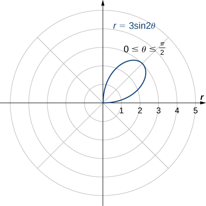
Reflecting this image into the other three quadrants gives the entire graph as shown.
Determine the symmetry of the graph determined by the equation \(r=2\,\text{cos}(3θ)\) and create a graph.
Symmetric with respect to the polar axis.
Key Concepts
- The polar coordinate system provides an alternative way to locate points in the plane. (See Example 2.)
- Convert points between rectangular and polar coordinates using the formulas
and\[x=r\,\text{cos}\,θ\,\text{and}\,y=r\,\text{sin}\,θ\]
\[r=\sqrt{{x}^{2}+{y}^{2}}\,\text{and}\,\text{tan}\,θ=\frac{y}{x}.\]
(See Example 1.) - To sketch a polar curve from a given polar function, make a table of values and take advantage of periodic properties. (See Example 3.)
- Use the conversion formulas to convert equations between rectangular and polar coordinates. (See Example 3 and Example 4.)
- Identify symmetry in polar curves, which can occur through the pole, the horizontal axis, or the vertical axis. (See Example 6.)
Section Exercises
In the following exercises, plot the point whose polar coordinates are given by first constructing the angle \(θ\) and then marking off the distance r along the ray.
\((3,\frac{\pi }{6})\)
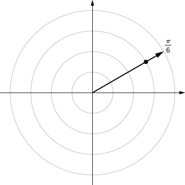
\((-2,\frac{5\pi }{3})\)
\((0,\frac{7\pi }{6})\)
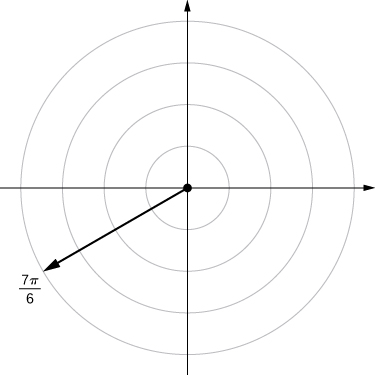
\((-4,\frac{3\pi }{4})\)
\((1,\frac{\pi }{4})\)
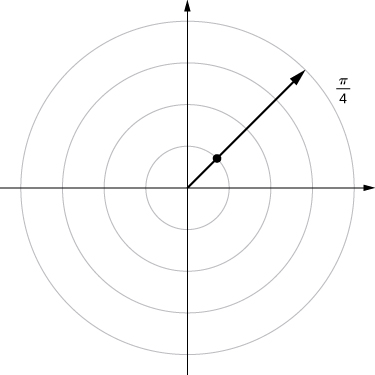
\((2,\frac{5\pi }{6})\)
\((1,\frac{\pi }{2})\)
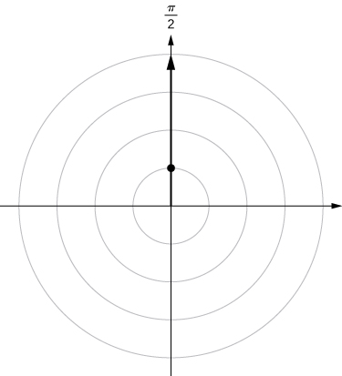
For the following exercises, consider the polar graph below. Give two sets of polar coordinates for each point.
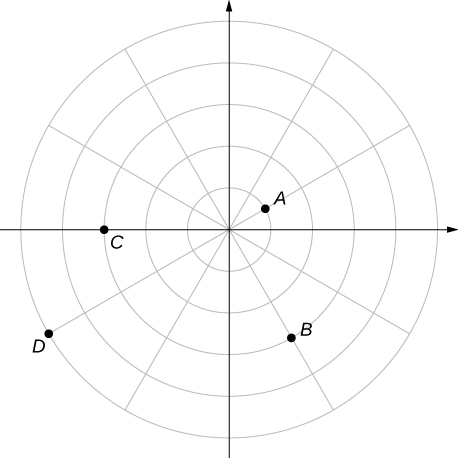
Coordinates of point A.
Coordinates of point B.
\(B\begin{array}{ll}(3,\frac{\text{-}\pi }{3}) & B(-3,\frac{2\pi }{3})\end{array}\)
Coordinates of point C.
Coordinates of point D.
\(D(5,\frac{7\pi }{6})D(-5,\frac{\pi }{6})\)
For the following exercises, the rectangular coordinates of a point are given. Find two sets of polar coordinates for the point in \((0,2\pi ].\) Round to three decimal places.
\((2,\,2)\)
\((3,-4)\)
\((5, 5.356) (-5, 2.214)\)
\((8,\,15)\)
\((-6,\,8)\)
\((10, 2.214)(-10, 5.356)\)
\((4,\,3)\)
\((3,\text{-}\sqrt{3})\)
\((2\sqrt{3},\frac{11\pi }{6})(-2\sqrt{3},\frac{5\pi }{6})\)
For the following exercises, find rectangular coordinates for the given point in polar coordinates.
\((2,\frac{5\pi }{4})\)
\((-2,\frac{\pi }{6})\)
\((\begin{array}{ll}\text{-}\sqrt{3}, & -1\end{array})\)
\((5,\frac{\pi }{3})\)
\((1,\frac{7\pi }{6})\)
\((\begin{array}{ll}-\frac{\sqrt{3}}{2}, & \frac{-1}{2}\end{array})\)
\((-3,\frac{3\pi }{4})\)
\((0,\frac{\pi }{2})\)
\((\begin{array}{ll}0, & 0\end{array})\)
\((-4.5,6.5)\)
For the following exercises, determine whether the graphs of the polar equation are symmetric with respect to the \(x\) -axis, the \(y\) -axis, or the origin.
\(r=3\,\text{sin}(2θ)\)
Symmetry with respect to the x-axis, y-axis, and origin.
\({r}^{2}=9\,\text{cos}\,θ\)
\(r=\text{cos}(\frac{θ}{5})\)
Symmetric with respect to x-axis only.
\(r=2\,\text{sec}\,θ\)
\(r=1+\text{cos}\,θ\)
Symmetry with respect to x-axis only.
For the following exercises, describe the graph of each polar equation. Confirm each description by converting into a rectangular equation.
\(r=3\)
\(θ=\frac{\pi }{4}\)
Line \(y=x\)
\(r=\text{sec}\,θ\)
\(r=\text{csc}\,θ\)
\(y=1\)
For the following exercises, convert the rectangular equation to polar form and sketch its graph.
\({x}^{2}+{y}^{2}=16\)
\({x}^{2}-{y}^{2}=16\)
Hyperbola; polar form \({r}^{2}\text{cos}(2θ)=16\) or \({r}^{2}=16\,\text{sec}\,(2θ).\)
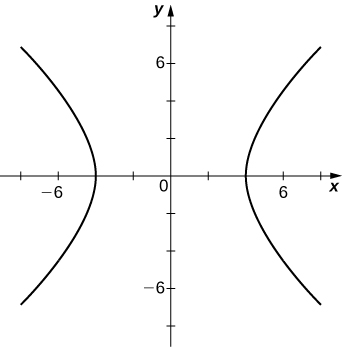
\(x=8\)
For the following exercises, convert the rectangular equation to polar form and sketch its graph.
\(3x-y=2\)
\(r=\frac{2}{3\,\text{cos}\,θ-\text{sin}\,θ}\)
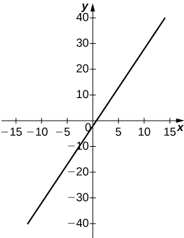
\({y}^{2}=4x\)
For the following exercises, convert the polar equation to rectangular form and sketch its graph.
\(r=4\,\text{sin}\,θ\)
\({x}^{2}+{y}^{2}=4y\)
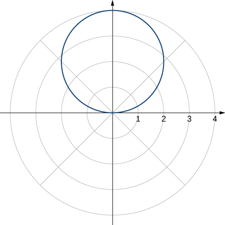
\(r=6\,\text{cos}\,θ\)
\(r=θ\)
\(x\,\text{tan}\sqrt{{x}^{2}+{y}^{2}}=y\)
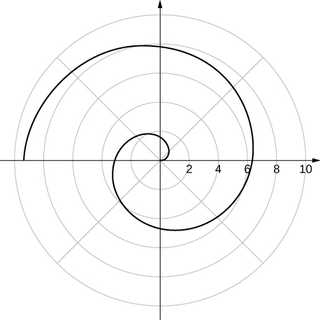
\(r=\text{cot}\,θ\,\text{csc}\,θ\)
For the following exercises, sketch a graph of the polar equation and identify any symmetry.
\(r=1+\text{sin}\,θ\)
y-axis symmetry
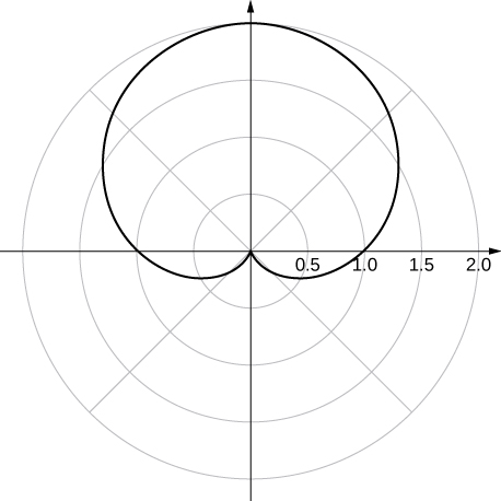
\(r=3-2\,\text{cos}\,θ\)
\(r=2-2\,\text{sin}\,θ\)
y-axis symmetry
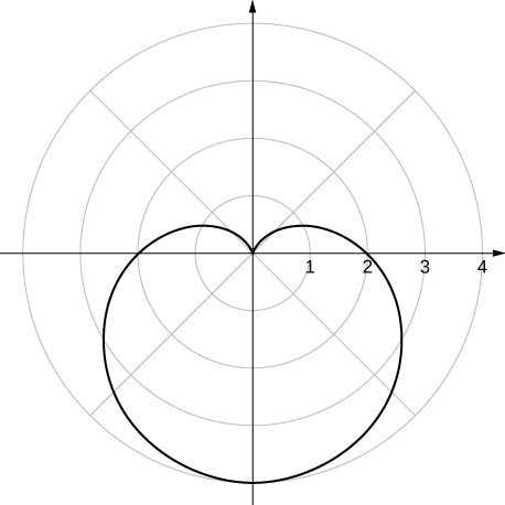
\(r=5-4\,\text{sin}\,θ\)
\(r=3\,\text{cos}(2θ)\)
x- and y-axis symmetry and symmetry about the pole
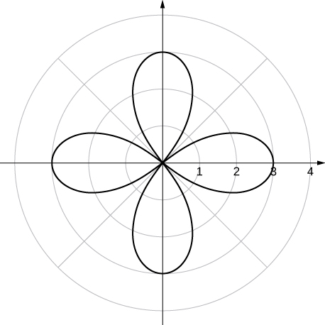
\(r=3\,\text{sin}(2θ)\)
\(r=2\,\text{cos}(3θ)\)
x-axis symmetry
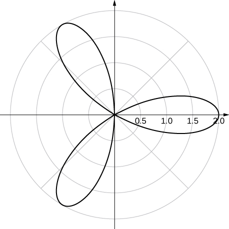
\(r=3\,\text{cos}(\frac{θ}{2})\)
\({r}^{2}=4\,\text{cos}(2θ)\)
x- and y-axis symmetry and symmetry about the pole
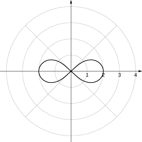
\({r}^{2}=4\,\text{sin}\,θ\)
\(r=2θ\)
no symmetry
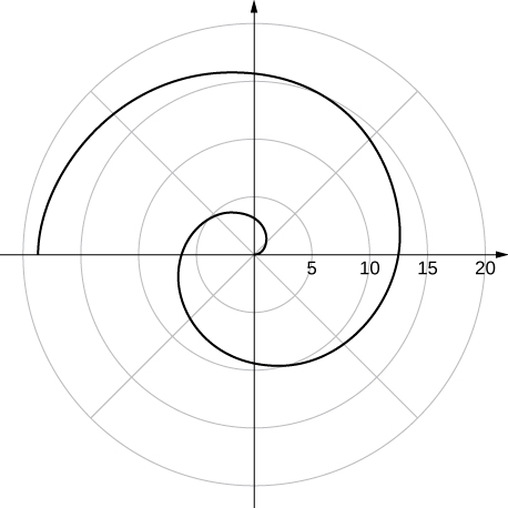
[T] The graph of \(r=2\,\text{cos}(2θ)\text{sec}(θ).\) is called a strophoid. Use a graphing utility to sketch the graph, and, from the graph, determine the asymptote.
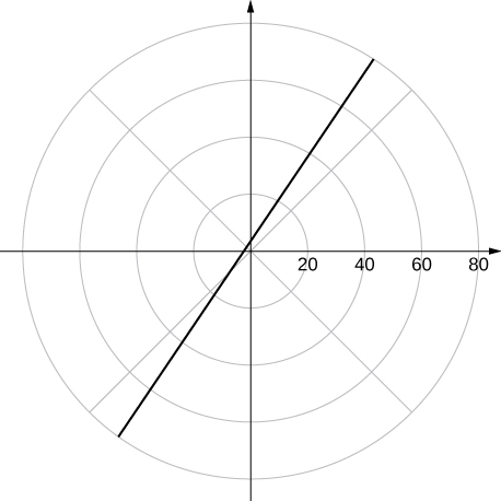
[T] Use a graphing utility and sketch the graph of \(r=\frac{6}{2\,\text{sin}\,θ-3\,\text{cos}\,θ}.\)
a line
[T] Use a graphing utility to graph \(r=\frac{1}{1-\text{cos}\,θ}.\)
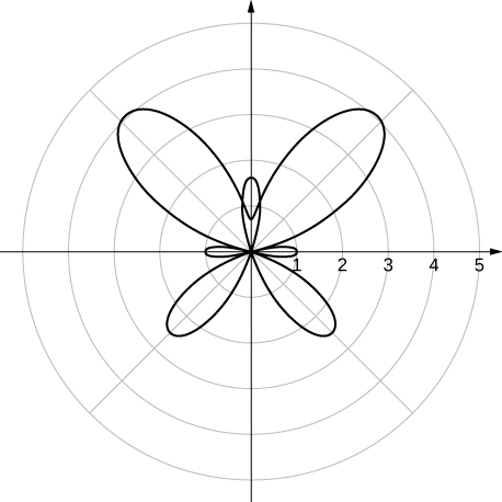
[T] Use technology to graph \(r={e}^{\text{sin}(θ)}-2\,\text{cos}(4θ).\)
[T] Use technology to plot \(r=\text{sin}(\frac{3θ}{7})\) (use the interval \(0\le θ\le 14\pi ).\)
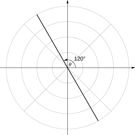
Without using technology, sketch the polar curve \(θ=\frac{2\pi }{3}.\)
[T] Use a graphing utility to plot \(r=θ\,\text{sin}\,θ\) for \(\text{-}\pi \le θ\le \pi .\)
[T] Use technology to plot \(r={e}^{-0.1θ}\) for \(-10\le θ\le 10.\)
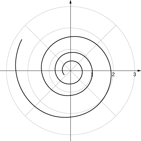
[T] There is a curve known as the “Black Hole.” Use technology to plot \(r={e}^{-0.01θ}\) for \(-100\le θ\le 100.\)
[T] Use the results of the preceding two problems to explore the graphs of \(r={e}^{-0.001θ}\) and \(r={e}^{-0.0001θ}\) for \(|θ|>100.\)
Answers vary. One possibility is the spiral lines become closer together and the total number of spirals increases.
Glossary
- angular coordinate
- \(θ\) the angle formed by a line segment connecting the origin to a point in the polar coordinate system with the positive radial (x) axis, measured counterclockwise
- cardioid
- a plane curve traced by a point on the perimeter of a circle that is rolling around a fixed circle of the same radius; the equation of a cardioid is \(r=a(1+\text{sin}\,θ)\) or \(r=a(1+\text{cos}\,θ)\)
- limaçon
- the graph of the equation \(r=a+b\,\text{sin}\,θ\) or \(r=a+b\,\text{cos}\,θ.\) If \(a=b\) then the graph is a cardioid
- polar axis
- the horizontal axis in the polar coordinate system corresponding to \(r\ge 0\)
- polar coordinate system
- a system for locating points in the plane. The coordinates are \(r,\) the radial coordinate, and \(θ,\) the angular coordinate
- polar equation
- an equation or function relating the radial coordinate to the angular coordinate in the polar coordinate system
- pole
- the central point of the polar coordinate system, equivalent to the origin of a Cartesian system
- radial coordinate
- \(r\) the coordinate in the polar coordinate system that measures the distance from a point in the plane to the pole
- rose
- graph of the polar equation \(r=a\,\text{cos}\,2θ\) or \(r=a\,\text{sin}\,2θ\) for a positive constant a
- space-filling curve
- a curve that completely occupies a two-dimensional subset of the real plane