Section 2.4Continuity

Many functions have the property that their graphs can be traced with a pencil without lifting the pencil from the page. Such functions are called continuous. Other functions have points at which a break in the graph occurs, but satisfy this property over intervals contained in their domains. They are continuous on these intervals and are said to have a discontinuity at a point where a break occurs.

We begin our investigation of continuity by exploring what it means for a function to have continuity at a point. Intuitively, a function is continuous at a particular point if there is no break in its graph at that point.

Continuity at a Point

Before we look at a formal definition of what it means for a function to be continuous at a point, let’s consider various functions that fail to meet our intuitive notion of what it means to be continuous at a point. We then create a list of conditions that prevent such failures.

Our first function of interest is shown in Figure 1. We see that the graph of \(f(x)\) has a hole at a. In fact, \(f(a)\) is undefined. At the very least, for \(f(x)\) to be continuous at a, we need the following condition:

\[\text{i.}\,f(a)\,\text{is defined.}\]

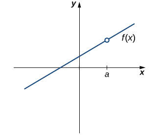
However, as we see in Figure 2, this condition alone is insufficient to guarantee continuity at the point a. Although \(f(a)\) is defined, the function has a gap at a. In this example, the gap exists because \(\underset{x\to a}{\text{lim}}f(x)\) does not exist. We must add another condition for continuity at a—namely,

\[\text{ii.}\,\underset{x\to a}{\text{lim}}f(x)\,\text{exists.}\]

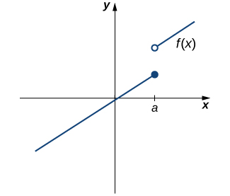
However, as we see in Figure 3, these two conditions by themselves do not guarantee continuity at a point. The function in this figure satisfies both of our first two conditions, but is still not continuous at a. We must add a third condition to our list:

\[\text{iii.}\,\underset{x\to a}{\text{lim}}f(x)=f(a).\]

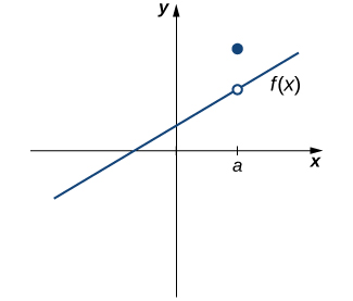
Now we put our list of conditions together and form a definition of continuity at a point.

The following procedure can be used to analyze the continuity of a function at a point using this definition.

The next three examples demonstrate how to apply this definition to determine whether a function is continuous at a given point. These examples illustrate situations in which each of the conditions for continuity in the definition succeed or fail.

Example 1

Using the definition, determine whether the function \(f(x)=({x}^{2}-4)\text{/}(x-2)\) is continuous at \(x=2.\) Justify the conclusion.

Try plugging x=2 into f directly — does that even make sense?

Show solution

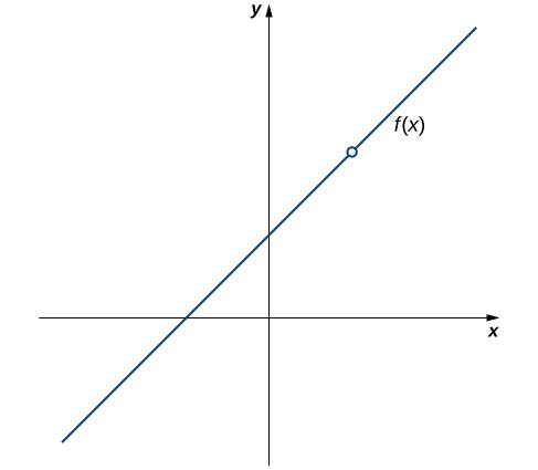
Let’s begin by trying to calculate \(f(2).\) We can see that \(f(2)=0\text{/}0,\) which is undefined. Therefore, \(f(x)=\frac{{x}^{2}-4}{x-2}\) is discontinuous at 2 because \(f(2)\) is undefined. The graph of \(f(x)\) is shown in Figure 4.

Example 2

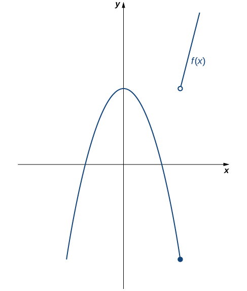
Using the definition, determine whether the function \(f(x)=\left\{\begin{array}{ll}-{x}^{2}+4 & \text{if}\,x\le 3 \\ 4x-8 & \text{if}\,x>3\end{array}\right.\) is continuous at \(x=3.\) Justify the conclusion.

Compute f(3) first, then check the two one-sided limits separately.

Show solution

Let’s begin by trying to calculate \(f(3).\)

\[f(3)=-({3}^{2})+4=-5.\]

Thus, \(f(3)\) is defined. Next, we calculate \(\underset{x\to 3}{\text{lim}}f(x).\) To do this, we must compute \(\underset{x\to {3}^{-}}{\text{lim}}f(x)\) and \(\underset{x\to {3}^{+}}{\text{lim}}f(x)\text{:}\)

\[\underset{x\to {3}^{-}}{\text{lim}}f(x)=-({3}^{2})+4=-5\]

and

\[\underset{x\to {3}^{+}}{\text{lim}}f(x)=4(3)-8=4.\]

Therefore, \(\underset{x\to 3}{\text{lim}}f(x)\) does not exist. Thus, \(f(x)\) is not continuous at 3. The graph of \(f(x)\) is shown in Figure 5.

By applying the definition of continuity and previously established theorems concerning the evaluation of limits, we can state the following theorem.

Proof

Previously, we showed that if \(p(x)\) and \(q(x)\) are polynomials, \(\underset{x\to a}{\text{lim}}p(x)=p(a)\) for every polynomial \(p(x)\) and \(\underset{x\to a}{\text{lim}}\frac{p(x)}{q(x)}=\frac{p(a)}{q(a)}\) as long as \(q(a)\ne 0.\) Therefore, polynomials and rational functions are continuous on their domains.

□

We now apply the theorem above to determine the points at which a given rational function is continuous.

Types of Discontinuities

As we have seen in Example 1 and Example 2, discontinuities take on several different appearances. We classify the types of discontinuities we have seen thus far as removable discontinuities, infinite discontinuities, or jump discontinuities. Intuitively, a removable discontinuity is a discontinuity for which there is a hole in the graph, a jump discontinuity is a noninfinite discontinuity for which the sections of the function do not meet up, and an infinite discontinuity is a discontinuity located at a vertical asymptote. Figure 6 illustrates the differences in these types of discontinuities. Although these terms provide a handy way of describing three common types of discontinuities, keep in mind that not all discontinuities fit neatly into these categories.

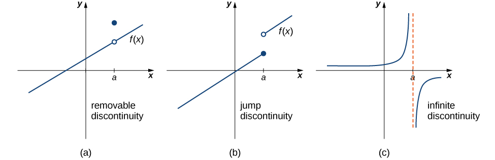
These three discontinuities are formally defined as follows:

Continuity over an Interval

Now that we have explored the concept of continuity at a point, we extend that idea to continuity over an interval. As we develop this idea for different types of intervals, it may be useful to keep in mind the intuitive idea that a function is continuous over an interval if we can use a pencil to trace the function between any two points in the interval without lifting the pencil from the paper. In preparation for defining continuity on an interval, we begin by looking at the definition of what it means for a function to be continuous from the right at a point and continuous from the left at a point.

A function is continuous over an open interval if it is continuous at every point in the interval. A function \(f(x)\) is continuous over a closed interval of the form \([a,b]\) if it is continuous at every point in \((a,b)\) and is continuous from the right at a and is continuous from the left at b. Analogously, a function \(f(x)\) is continuous over an interval of the form \((a,b]\) if it is continuous over \((a,b)\) and is continuous from the left at b. Continuity over other types of intervals are defined in a similar fashion.

Requiring that \(\underset{x\to {a}^{+}}{\text{lim}}f(x)=f(a)\) and \(\underset{x\to {b}^{-}}{\text{lim}}f(x)=f(b)\) ensures that we can trace the graph of the function from the point \((a,f(a))\) to the point \((b,f(b))\) without lifting the pencil. If, for example, \(\underset{x\to {a}^{+}}{\text{lim}}f(x)\ne f(a),\) we would need to lift our pencil to jump from \(f(a)\) to the graph of the rest of the function over \((a,b].\)

The composite function theorem below allows us to expand our ability to compute limits. In particular, this theorem ultimately allows us to demonstrate that trigonometric functions are continuous over their domains.

Before we move on to Example 10, recall that earlier, in the section on limit laws, we showed \(\underset{x\to 0}{\text{lim}}\,\text{cos}\,x=1=\text{cos}\,(0).\) Consequently, we know that \(f(x)=\text{cos}\,x\) is continuous at 0. In Example 10 we see how to combine this result with the composite function theorem.

The proof of the next theorem uses the composite function theorem as well as the continuity of \(f(x)=\text{sin}\,x\) and \(g(x)=\text{cos}\,x\) at the point 0 to show that trigonometric functions are continuous over their entire domains.

Proof

We begin by demonstrating that \(\text{cos}\,x\) is continuous at every real number. To do this, we must show that \(\underset{x\to a}{\text{lim}}\text{cos}\,x=\text{cos}\,a\) for all values of a.

\(\begin{array}{lllll}\underset{x\to a}{\text{lim}}\text{cos}\,x & =\underset{x\to a}{\text{lim}}\text{cos}\,((x-a)+a) & & & \text{rewrite}\,x=x-a+a \\ & =\underset{x\to a}{\text{lim}}(\text{cos}\,(x-a)\,\text{cos}\,a-\text{sin}\,(x-a)\,\text{sin}\,a) & & & \text{apply the identity for the cosine of the sum of two angles} \\ & =\text{cos}\,(\underset{x\to a}{\text{lim}}(x-a))\,\text{cos}\,a-\text{sin}\,(\underset{x\to a}{\text{lim}}(x-a))\,\text{sin}\,a & & & \underset{x\to a}{\text{lim}}(x-a)=0,\,\text{and}\,\text{sin}\,x\,\text{and}\,\text{cos}\,x\,\text{are continuous at 0} \\ & =\text{cos}\,(0)\,\text{cos}\,a-\text{sin}\,(0)\,\text{sin}\,a & & & \text{evaluate cos(0) and sin(0) and simplify} \\ & =1·\text{cos}\,a-0·\text{sin}\,a=\text{cos}\,a.\end{array}\)

The proof that \(\text{sin}\,x\) is continuous at every real number is analogous. Because the remaining trigonometric functions may be expressed in terms of \(\text{sin}\,x\) and \(\text{cos}\,x,\) their continuity follows from the quotient limit law.

□

As you can see, the composite function theorem is invaluable in demonstrating the continuity of trigonometric functions. As we continue our study of calculus, we revisit this theorem many times.

The Intermediate Value Theorem

Functions that are continuous over intervals of the form \([a,b],\) where a and b are real numbers, exhibit many useful properties. Throughout our study of calculus, we will encounter many powerful theorems concerning such functions. The first of these theorems is the Intermediate Value Theorem.

The Intermediate Value Theorem

Let f be continuous over a closed, bounded interval \([a,b].\) If z is any real number between \(f(a)\) and \(f(b),\) then there is a number c in \([a,b]\) satisfying \(f(c)=z\) in Figure 7.

Key Concepts

• For a function to be continuous at a point, it must be defined at that point, its limit must exist at the point, and the value of the function at that point must equal the value of the limit at that point.
• Discontinuities may be classified as removable, jump, or infinite.
• A function is continuous over an open interval if it is continuous at every point in the interval. It is continuous over a closed interval if it is continuous at every point in its interior and is continuous at its endpoints.
• The composite function theorem states: If \(f(x)\) is continuous at L and \(\underset{x\to a}{\text{lim}}g(x)=L,\) then \(\underset{x\to a}{\text{lim}}f(g(x))=f(\underset{x\to a}{\text{lim}}g(x))=f(L).\)
• The Intermediate Value Theorem guarantees that if a function is continuous over a closed interval, then the function takes on every value between the values at its endpoints.

Section Exercises

For the following exercises, determine the point(s), if any, at which each function is discontinuous. Classify any discontinuity as jump, removable, infinite, or other.

1

\(f(x)=\frac{1}{\sqrt{x}}\)

Show answer

The function is defined for all x in the interval \((0,\infty ).\)

2

\(f(x)=\frac{2}{{x}^{2}+1}\)

3

\(f(x)=\frac{x}{{x}^{2}-x}\)

Show answer

Removable discontinuity at \(x=0;\) infinite discontinuity at \(x=1\)

4

\(g(t)={t}^{-1}+1\)

5

\(f(x)=\frac{5}{{e}^{x}-2}\)

Show answer

Infinite discontinuity at \(x=\text{ln}\,2\)

6

\(f(x)=\frac{|x-2|}{x-2}\)

7

\(H(x)=\text{tan}\,2x\)

Show answer

Infinite discontinuities at \(x=\frac{(2k+1)\pi }{4},\) for \(k=0,\pm 1,\pm 2,\pm 3\text{,…}\)

8

\(f(t)=\frac{t+3}{{t}^{2}+5t+6}\)

For the following exercises, decide if the function continuous at the given point. If it is discontinuous, what type of discontinuity is it?

9

\(f(x)=\frac{2{x}^{2}-5x+3}{x-1}\) at \(x=1\)

Show answer

No. It is a removable discontinuity.

10

\(h(θ)=\frac{\text{sin}\,θ-\text{cos}\,θ}{\text{tan}\,θ}\) at \(θ=\pi\)

11

\(g(u)=\left\{\begin{array}{ll}\frac{6{u}^{2}+u-2}{2u-1} & \text{if}\,u\ne \frac{1}{2} \\ \frac{7}{2} & \text{if}\,u=\frac{1}{2}\end{array}\right.,\) at \(u=\frac{1}{2}\)

Show answer

Yes. It is continuous.

12

\(f(y)=\frac{\text{sin}\,(\pi y)}{\text{tan}\,(\pi y)},\) at \(y=1\)

13

\(f(x)=\left\{\begin{array}{ll}{x}^{2}-{e}^{x} & \text{if}\,x<0 \\ x-1 & \text{if}\,x\ge 0\end{array}\right.,\) at \(x=0\)

Show answer

Yes. It is continuous.

14

\(f(x)=\left\{\begin{array}{l}x\,\text{sin}\,(x)\,\text{if}\,x\le \pi \\ x\,\text{tan}\,(x)\,\text{if}\,x>\pi \end{array}\right.,\) at \(x=\pi\)

In the following exercises, find the value(s) of k that makes each function continuous over the given interval.

15

\(f(x)=\left\{\begin{array}{ll}3x+2, & x<k \\ 2x-3, & k\le x\le 8\end{array}\right.\)

Show answer

\(k=-5\)

16

\(f(θ)=\left\{\begin{array}{ll}\text{sin}\,θ, & 0\le θ<\frac{\pi }{2} \\ \text{cos}\,(θ+k), & \frac{\pi }{2}\le θ\le \pi \end{array}\right.\)

17

\(f(x)=\left\{\begin{array}{ll}\frac{{x}^{2}+3x+2}{x+2}, & x\ne -2 \\ k, & x=-2\end{array}\right.\)

Show answer

\(k=-1\)

18

\(f(x)=\left\{\begin{array}{ll}{e}^{kx}, & 0\le x<4 \\ x+3, & 4\le x\le 8\end{array}\right.\)

19

\(f(x)=\left\{\begin{array}{ll}\sqrt{kx}, & 0\le x\le 3 \\ x+1, & 3<x\le 10\end{array}\right.\)

Show answer

\(k=\frac{16}{3}\)

In the following exercises, use the Intermediate Value Theorem (IVT).

20

Let \(h(x)=\left\{\begin{array}{ll}3{x}^{2}-4, & x\le 2 \\ 5+4x, & x>2\end{array}\right.\) Over the interval \([0,4],\) there is no value of x such that \(h(x)=10,\) although \(h(0)<10\) and \(h(4)>10.\) Explain why this does not contradict the IVT.

21

A particle moving along a line has at each time t a position function \(s(t),\) which is continuous. Assume \(s(2)=5\) and \(s(5)=2.\) Another particle moves such that its position is given by \(h(t)=s(t)-t.\) Explain why there must be a value c for \(2<c<5\) such that \(h(c)=0.\)

Show answer

Since both s and \(y=t\) are continuous everywhere, then \(h(t)=s(t)-t\) is continuous everywhere and, in particular, it is continuous over the closed interval \([2,5].\) Also, \(h(2)=3>0\) and \(h(5)=-3<0.\) Therefore, by the IVT, there is a value \(x=c\) such that \(h(c)=0.\)

22

[T] Use the statement “The cosine of t is equal to t cubed.”

• Write a mathematical equation of the statement.
• Prove that the equation in part a. has at least one real solution.
• Use a calculator to find an interval of length 0.01 that contains a solution.

23

Apply the IVT to determine whether \({2}^{x}={x}^{3}\) has a solution in one of the intervals \([1.25,1.375]\) or \([1.375,1.5].\) Briefly explain your response for each interval.

Show answer

The function \(f(x)={2}^{x}-{x}^{3}\) is continuous over the interval \([1.25,1.375]\) and has opposite signs at the endpoints.

24

Consider the graph of the function \(y=f(x)\) shown in the following graph.

• Find all values for which the function is discontinuous.
• For each value in part a., state why the formal definition of continuity does not apply.
• Classify each discontinuity as either jump, removable, or infinite.

25

Let \(f(x)=\left\{\begin{array}{l}3x,x>1 \\ {x}^{3},x<1\end{array}\right..\)

• Sketch the graph of f.
• Is it possible to find a value k such that \(f(1)=k,\) which makes \(f(x)\) continuous for all real numbers? Briefly explain.

Show answer

a.
1. It beings with an open circle at (1,3).">
b. It is not possible to redefine \(f(1)\) since the discontinuity is a jump discontinuity.

26

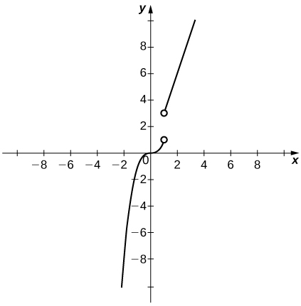
Let \(f(x)=\frac{{x}^{4}-1}{{x}^{2}-1}\) for \(x\ne -1,1.\)

• Sketch the graph of f.
• Is it possible to find values \({k}_{1}\) and \({k}_{2}\) such that \(f(-1)={k}_{1}\) and \(f(1)={k}_{2},\) and that makes \(f(x)\) continuous for all real numbers? Briefly explain.

27

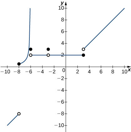
Sketch the graph of a function \(y=f(x)\) with properties i. through vi.

• The domain of f is \((\text{-}\infty ,\text{+}\infty ).\)
• f has an infinite discontinuity at \(x=-6.\)
• \(f(-6)=3\)
• \(\underset{x\to {-3}^{-}}{\text{lim}}f(x)=\underset{x\to {-3}^{+}}{\text{lim}}f(x)=2\)
• \(f(-3)=3\)
• f is left continuous but not right continuous at \(x=3.\)

Show answer

Answers may vary; see the following example:
3.">

28

Sketch the graph of a function \(y=f(x)\) with properties i. through iv.

• The domain of f is \([0,5].\)
• \(\underset{x\to {1}^{+}}{\text{lim}}f(x)\) and \(\underset{x\to {1}^{-}}{\text{lim}}f(x)\) exist and are equal.
• \(f(x)\) is left continuous but not continuous at \(x=2,\) and right continuous but not continuous at \(x=3.\)
• \(f(x)\) has a removable discontinuity at \(x=1,\) a jump discontinuity at \(x=2,\) and the following limits hold: \(\underset{x\to {3}^{-}}{\text{lim}}f(x)=\text{-}\infty\) and \(\underset{x\to {3}^{+}}{\text{lim}}f(x)=2.\)

In the following exercises, suppose \(y=f(x)\) is defined for all x. For each description, sketch a graph with the indicated property.

29

Discontinuous at \(x=1\) with \(\underset{x\to -1}{\text{lim}}f(x)=-1\) and \(\underset{x\to 2}{\text{lim}}f(x)=4\)

Show answer

Answers may vary; see the following example:
1. It begins at (1,3).">

30

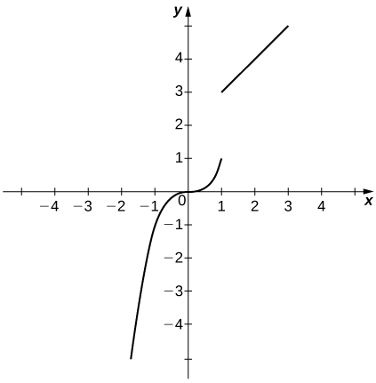
Discontinuous at \(x=2\) but continuous elsewhere with \(\underset{x\to 0}{\text{lim}}f(x)=\frac{1}{2}\)

Determine whether each of the given statements is true. Justify your response with an explanation or counterexample.

31

\(f(t)=\frac{2}{{e}^{t}-{e}^{-t}}\) is continuous everywhere.

Show answer

False. It is continuous over \((\text{-}\infty ,0)∪(0,\infty ).\)

32

If the left- and right-hand limits of \(f(x)\) as \(x\to a\) exist and are equal, then f cannot be discontinuous at \(x=a.\)

33

If a function is not continuous at a point, then it is not defined at that point.

Show answer

False. Consider \(f(x)=\left\{\begin{array}{l}x\,\text{if}\,x\ne 0 \\ 4\,\text{if}\,x=0\end{array}\right..\)

34

According to the IVT, \(\text{cos}\,x-\text{sin}\,x-x=2\) has a solution over the interval \([-1,1].\)

35

If \(f(x)\) is continuous such that \(f(a)\) and \(f(b)\) have opposite signs, then \(f(x)=0\) has exactly one solution in \([a,b].\)

Show answer

False. IVT only says that there is at least one solution; it does not guarantee that there is exactly one. Consider \(f(x)=\text{cos}\,(x)\) on \([-\pi ,2\pi ].\)

36

The function \(f(x)=\frac{{x}^{2}-4x+3}{{x}^{2}-1}\) is continuous over the interval \([0,3].\)

37

If \(f(x)\) is continuous everywhere and \(f(a),f(b)>0,\) then there is no root of \(f(x)\) in the interval \([a,b].\)

Show answer

False. The IVT does not work in reverse! Consider \({(x-1)}^{2}\) over the interval \([-2,2].\)

[T] The following problems consider the scalar form of Coulomb’s law, which describes the electrostatic force between two point charges, such as electrons. It is given by the equation \(F(r)={k}_{e}\frac{|{q}_{1}{q}_{2}|}{{r}^{2}},\) where \({k}_{e}\) is Coulomb’s constant, \({q}_{i}\) are the magnitudes of the charges of the two particles, and r is the distance between the two particles.

38

To simplify the calculation of a model with many interacting particles, after some threshold value \(r=R,\) we approximate F as zero.

• Explain the physical reasoning behind this assumption.
• What is the force equation?
• Evaluate the force F using both Coulomb’s law and our approximation, assuming two protons with a charge magnitude of \(1.6022\,\times \,{10}^{-19}\,\text{coulombs (C)},\) and the Coulomb constant \({k}_{e}=8.988\,\times \,{10}^{9}{\text{Nm}}^{2}\text{/}{\text{C}}^{2}\) are 1 m apart. Also, assume \(R<1\,\text{m}.\) How much inaccuracy does our approximation generate? Is our approximation reasonable?
• Is there any finite value of R for which this system remains continuous at R?

39

Instead of making the force 0 at R, instead we let the force be 10⁻²⁰ for \(r\ge R.\) Assume two protons, which have a magnitude of charge \(1.6022\,\times \,{10}^{-19}\,\text{C},\) and the Coulomb constant \({k}_{e}=8.988\,\times \,{10}^{9}{\text{Nm}}^{2}\text{/}{\text{C}}^{2}.\) Is there a value R that can make this system continuous? If so, find it.

Show answer

\(R=0.0001519\,\text{m}\)

Recall the discussion on spacecraft from the chapter opener. The following problems consider a rocket launch from Earth’s surface. The force of gravity on the rocket is given by \(F(d)=-mk\text{/}{d}^{2},\) where m is the mass of the rocket, d is the distance of the rocket from the center of Earth, and k is a constant.

40

[T] Determine the value and units of k given that the mass of the rocket is 3 million kg. (Hint: The distance from the center of Earth to its surface is 6378 km.)

41

[T] After a certain distance D has passed, the gravitational effect of Earth becomes quite negligible, so we can approximate the force function by \(F(d)=\left\{\begin{array}{ll}-\frac{mk}{{d}^{2}} & \text{if}\,d<D \\ 10,000 & \text{if}\,d\ge D\end{array}\right..\) Using the value of k found in the previous exercise, find the necessary condition D such that the force function remains continuous.

Show answer

\(D=345,826\,\text{km}\)

42

As the rocket travels away from Earth’s surface, there is a distance D where the rocket sheds some of its mass, since it no longer needs the excess fuel storage. We can write this function as \(F(d)=\left\{\begin{array}{l}-\frac{{m}_{1}k}{{d}^{2}}\,\text{if}\,d<D \\ -\frac{{m}_{2}k}{{d}^{2}}\,\text{if}\,d\ge D\end{array}\right..\) Is there a D value such that this function is continuous, assuming \({m}_{1}\ne {m}_{2}?\)

Prove the following functions are continuous everywhere

43

\(f(θ)=\text{sin}\,θ\)

Show answer

For all values of \(a,f(a)\) is defined, \(\underset{θ\to a}{\text{lim}}f(θ)\) exists, and \(\underset{θ\to a}{\text{lim}}f(θ)=f(a).\) Therefore, \(f(θ)\) is continuous everywhere.

44

\(g(x)=|x|\)

45

Where is \(f(x)=\left\{\begin{array}{l}0\,\text{if}\,x\,\text{is irrational} \\ 1\,\text{if}\,x\,\text{is rational}\end{array}\right.\) continuous?

Show answer

Nowhere

Glossary

continuity at a point

A function \(f(x)\) is continuous at a point a if and only if the following three conditions are satisfied: (1) \(f(a)\) is defined, (2) \(\underset{x\to a}{\text{lim}}f(x)\) exists, and (3) \(\underset{x\to a}{\text{lim}}f(x)=f(a)\)

continuity from the left

A function is continuous from the left at b if \(\underset{x\to {b}^{-}}{\text{lim}}f(x)=f(b)\)

continuity from the right

A function is continuous from the right at a if \(\underset{x\to {a}^{+}}{\text{lim}}f(x)=f(a)\)

continuity over an interval

a function that can be traced with a pencil without lifting the pencil; a function is continuous over an open interval if it is continuous at every point in the interval; a function \(f(x)\) is continuous over a closed interval of the form \([a,b]\) if it is continuous at every point in \((a,b),\) and it is continuous from the right at a and from the left at b

discontinuity at a point

A function is discontinuous at a point or has a discontinuity at a point if it is not continuous at the point

infinite discontinuity

An infinite discontinuity occurs at a point a if \(\underset{x\to {a}^{-}}{\text{lim}}f(x)=\text{±}\infty\) or \(\underset{x\to {a}^{+}}{\text{lim}}f(x)=\text{±}\infty\)

Intermediate Value Theorem

Let f be continuous over a closed bounded interval \([\text{a},\text{b}];\) if z is any real number between \(f(a)\) and \(f(b),\) then there is a number c in \([a,b]\) satisfying \(f(c)=z\)

jump discontinuity

A jump discontinuity occurs at a point a if \(\underset{x\to {a}^{-}}{\text{lim}}f(x)\) and \(\underset{x\to {a}^{+}}{\text{lim}}f(x)\) both exist, but \(\underset{x\to {a}^{-}}{\text{lim}}f(x)\ne \underset{x\to {a}^{+}}{\text{lim}}f(x)\)

removable discontinuity

A removable discontinuity occurs at a point a if \(f(x)\) is discontinuous at a, but \(\underset{x\to a}{\text{lim}}f(x)\) exists