How can a definite integral be used to measure the length of a
curve in 2- or 3-space?
Why is arc length useful as a parameter?
What is the curvature of a curve?
Given a space curve, there are two natural
geometric questions one might ask: how long is the curve and how much
does it bend? In this section, we answer both questions by
developing techniques for measuring the length of a space
curve as well as its curvature.
Preview Activity 9.8.1
In earlier investigations, we have used
integration to calculate quantities such as area, volume, mass, and
work. We are now interested in determining the
length of a space curve.
Consider the smooth curve in 3-space defined by the vector-valued
function \(\vr\), where
\[
\vr(t) = \langle x(t), y(t), z(t) \rangle = \langle \cos(t), \sin(t), t \rangle
\]
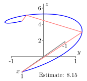
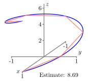
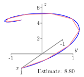
for \(t\) in the interval \([0,2\pi]\). Pictures of the graph of \(\vr\) are shown in Figure 9.8.1.
We will use the integration process to calculate the length of this curve. In this situation we partition the interval \([0,2\pi]\) into \(n\) subintervals of equal length and let \(0 = t_0 \lt t_1 \lt t_2 \lt \cdots \lt t_n = b\) be the endpoints of the subintervals. We then approximate the length of the curve on each subinterval with some related quantity that we can compute. In this case, we approximate the length of the curve on each subinterval with the length of the segment connecting the endpoints. Figure 9.8.1 illustrates the process in three different instances using increasing values of \(n\).
Figure 9.8.1 — Approximating the length of the curve with \(n=3\), \(n=6\), and \(n=9\).
Write a formula for the length of the line segment that connects the endpoints of the curve on the \(i\)th subinterval \([t_{i-1},t_i]\). (This length is our approximation of the length of the curve on this interval.)
Use your formula in part (a) to write a sum that adds all of the approximations to the lengths on each subinterval.
What do we need to do with the sum in part (b) in order to obtain the exact value of the length of the graph of \(\vr(t)\) on the interval \([0,2\pi]\)?
Arc Length
Consider a smooth curve in 3-space that is parametrically described by
the vector-valued function \(\vr\) defined by \(\vr(t) = \langle x(t), y(t), z(t)
\rangle.\)
Preview Activity 9.8.1 shows that to approximate the
length of the curve defined by \(\vr(t)\) as the values of \(t\) run over
an interval \([a,b]\), we partition the interval \([a,b]\) into \(n\)
subintervals of equal length \(\Delta t\), with \(a = t_0 \lt t_1 \lt \cdots
\lt t_n = b\) as the endpoints of the subintervals. On each subinterval,
we approximate the length of the curve by the length of the line
segment connecting the endpoints. The points on the curve
corresponding to \(t = t_{i-1}\) and \(t = t_i\) are \((x(t_{i-1}),
y(t_{i-1}), z(t_{i-1}))\) and \((x(t_i), y(t_i), z(t_i))\), respectively,
so the length of the line segment connecting these points is
\[
\sqrt{(x(t_i) - x(t_{i-1}))^2 + (y(t_i) - y(t_{i-1}))^2 + (z(t_i) -
z(t_{i-1}))^2}.
\]
Now we add all of these approximations together to obtain an
approximation to the length \(L\) of the curve:
\[
L \approx \sum_{i=1}^n \sqrt{(x(t_i) - x(t_{i-1}))^2 + (y(t_i) -
y(t_{i-1}))^2 + (z(t_i) - z(t_{i-1}))^2}.
\]
We now want to take the limit of this sum as \(n\) goes to infinity, but in its present form it
might be difficult to see how. We first introduce \(\Delta t\) by multiplying by \(\frac{\Delta t}{\Delta t}\), and see that
\[\begin{aligned}L & \approx \sum_{i=1}^n \sqrt{(x(t_i) - x(t_{i-1}))^2 + (y(t_i) - y(t_{i-1}))^2 + (z(t_i) - z(t_{i-1}))^2} \\
& = \sum_{i=1}^n \sqrt{(x(t_i) - x(t_{i-1}))^2 + (y(t_i) - y(t_{i-1}))^2 + (z(t_i) - z(t_{i-1}))^2} \frac{\Delta t}{\Delta t} \\
& = \sum_{i=1}^n \sqrt{(x(t_i) - x(t_{i-1}))^2 + (y(t_i) - y(t_{i-1}))^2 + (z(t_i) - z(t_{i-1}))^2} \frac{\Delta t}{\sqrt{(\Delta t)^2}}\end{aligned}\]
To get the difference quotients under the radical, we use properties of the square root function to see further that
\[\begin{aligned}L & \approx \sum_{i=1}^n \sqrt{\left[(x(t_i) - x(t_{i-1}))^2 + (y(t_i) - y(t_{i-1}))^2 + (z(t_i) - z(t_{i-1})^2\right] \frac{1}{(\Delta t)^2}} \Delta t \\
& = \sum_{i=1}^n \sqrt{\left(\frac{x(t_i) - x(t_{i-1})}{\Delta t}\right)^2 + \left(\frac{y(t_i) - y(t_{i-1})}{\Delta t}\right)^2 + \left(\frac{z(t_i) - z(t_{i-1})}{\Delta t}\right)^2} \Delta t.\end{aligned}\]
Recall that as \(n \to \infty\) we also have \(\Delta t \to 0\). Since
\[\begin{aligned} x'(t) & = \lim_{\Delta t \to 0} \frac{x(t_i) - x(t_{i-1})}{\Delta t}, \\
y'(t) & = \lim_{\Delta t \to 0} \frac{y(t_i) - y(t_{i-1})}{\Delta t}, \ \text{ and } \\
z'(t) & \lim_{\Delta t \to 0} \frac{z(t_i) - z(t_{i-1})}{\Delta t}, \end{aligned}\]
we see that
\[\lim_{n \to \infty} \sum_{i=1}^n \sqrt{\left(\frac{x(t_i) - x(t_{i-1})}{\Delta t}\right)^2 + \left(\frac{y(t_i) - y(t_{i-1})}{\Delta t}\right)^2 + \left(\frac{z(t_i) - z(t_{i-1})}{\Delta t}\right)^2} \Delta t
\]
is equal to
\[
\int_a^b \sqrt{(x'(t))^2 + (y'(t))^2 + (z'(t))^2} \, dt.
\]
Noting further that
\[
|\vr'(t)| = \sqrt{(x'(t))^2 + (y'(t))^2 + (z'(t))^2},
\]
we can rewrite our arclength formula in a more succinct form as follows.
The length of a curve
If \(\vr(t)\) defines a smooth curve \(C\) on an interval \([a,b]\), then the length \(L\) of \(C\) is given by
\[
L = \int_a^b |\vr'(t)| \, dt.
\tag{9.8.1}\]
Note that formula (9.8.1) applies to curves in any
dimensional space. Moreover, this formula has a natural interpretation: if
\(\vr(t)\) records the position of a moving object, then \(\vr'(t)\) is
the object's velocity and \(|\vr'(t)|\) its speed. Formula
(9.8.1) says that we simply integrate the speed of
an object traveling over the curve to find the distance traveled by
the object, which is the same as the length of the curve,
just as in one-variable calculus.
Activity 9.8.2
Here we calculate the arc length of two familiar curves.
Use Equation (9.8.1) to calculate the circumference of a circle of radius \(r\).
Find the exact length of the spiral defined by \(\vr(t) = \langle \cos(t), \sin(t), t \rangle\) on the interval \([0,2\pi]\).
We can adapt the arc length formula to curves in 2-space that define
\(y\) as a function of \(x\) as the following activity shows.
Activity 9.8.3
Let \(y = f(x)\) define a smooth curve in 2-space. Parameterize this curve and use Equation (9.8.1) to show that the length of the curve defined by \(f\) on an interval \([a,b]\) is
\[
\int_a^b \sqrt{1+[f'(t)]^2} \, dt.
\]
Parameterizing With Respect To Arc Length
In addition to helping us to find the length of space curves, the
expression for the length of a curve enables us to find a natural
parametrization of space curves in terms of arc length, as we now
explain.
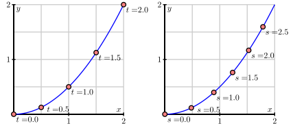
Shown below in Figure 9.8.2 is a portion of the
parabola \(y = x^2/2\). Of course, this space curve may be parametrized by
the vector-valued function \(\vr\) defined by \(\vr(t) = \langle t, t^2/2\rangle\) as shown
on the left, where we see the location at a few different times \(t\).
Notice that the points are not equally spaced on the curve.
A more natural parameter describing the points along the space curve
is the distance traveled \(s\) as we move along the parabola starting at
the origin. For instance, the right side of Figure 9.8.2 shows the points corresponding to various
values of \(s\). We call this an arc length parametrization.
Figure 9.8.2 — The parametrization \(\vr(t)\) (left) and a
reparametrization by arc length.
To see that this is a more natural parametrization, consider an
interstate highway cutting across a state. One way
to parametrize the curve defined by the highway is to drive along the
highway and record our position at every time, thus creating a
function \(\vr\). If we encounter an accident or road construction,
however,
this parametrization might not be at all relevant to another person
driving the same highway. An arc length parametrization, however, is
like using the mile markers on the side of road to specify our
position on the highway. If we know how far we've traveled along the
highway, we know exactly where we are.
If we begin with a parametrization of a space curve, we can
modify it to find an arc length parametrization, as we now describe.
Suppose that the curve is parametrized by the vector-valued function
\(\vr = \vr(t)\) where \(t\) is in the interval \([a,b]\). We define the
parameter \(s\) through the function
\[
s=L(t) = \int_a^t \sqrt{(x'(w))^2 + (y'(w))^2 + (z'(w))^2} \,dw,
\]
which measures the length along the curve from \(\vr(a)\) to
\(\vr(t)\).
The Fundamental Theorem of Calculus shows us that
\[
\frac{ds}{dt} =
L'(t)=
\sqrt{(x'(t))^2 + (y'(t))^2 + (z'(t))^2} = \text{|} \vr'(t) \text{|}
\tag{9.8.2}\]
and so
\[
L(t) = \int_a^t \left\lvert \frac{d}{dw}\vr(w)\right\rvert \,dw.
\]
If we assume that \(\vr'(t)\) is never 0, then \(L'(t) > 0\) for all \(t\)
and \(s=L(t)\) is always increasing. This should seem reasonable: unless we
stop, the distance traveled along the curve increases as we move along
the curve.
Since \(s=L(t)\) is an increasing function, it is invertible, which means
we may view the time \(t\) as a function of the distance traveled; that
is, we have the relationship \(t=L^{-1}(s)\). We then obtain the arc length
parametrization by composing \(\vr(t)\) with \(t=L^{-1}(s)\) to obtain
\(\vr(s)\). Let's illustrate this with an example.
Example 9.8.1
Consider a circle of
radius \(5\) in 2-space centered at the origin. We know that we can
parameterize this circle as
\[
\vr(t) = \langle 5\cos(t), 5\sin(t) \rangle,
\]
where \(t\) runs from 0 to \(2\pi\).
We see that \(\vr'(t) = \langle -5\sin(t), 5\cos(t) \rangle\), and hence
\(|\vr'(t)| = 5\). It then follows that
\[
s=L(t) = \int_0^t |\vr'(w)|~dw = \int_0^t 5~dw = 5t.
\]
Since \(s=L(t) = 5t\), we may solve for \(t\) in terms of \(s\) to obtain
\(t(s)=L^{-1}(s)
= s/5\). We then find the arc length parametrization by composing
\[
\vr(t(s))=\vr(L^{-1}(s)) = \left\langle 5\cos\left(\frac s5\right),
5\sin\left(\frac s5\right)\right\rangle.
\]
More generally, for a circle of radius \(a\) centered at the origin, a
similar computation shows that
\[
\left\langle a\cos\left(\frac sa\right), a\sin\left(\frac sa\right)\right\rangle
\tag{9.8.3}\]
is an arc length parametrization.
Notice that equation (9.8.2) shows that
\[
\frac{d\vr}{dt} = \frac{d\vr}{ds}\frac{ds}{dt} = \frac{d\vr}{ds}\text{|} \vr'(t) \text{|},
\]
so
\[
\left\lvert \frac{d\vr}{ds} \right\rvert = \left\lvert\frac{1}{\text{|} \vr'(t) \text{|}}\frac{d\vr}{dt} \right\rvert = 1,
\]
which means that we move along the curve with unit speed when we parameterize by arc length. This is clearly seen in Example 9.8.1 where \(|\vr'(s)| = 1\). It follows that the parameter \(s\)
is the distance traveled along the curve, as shown by:
\[
L(s) = \int_0^s\left\lvert\frac{d}{ds}\vr(w)\right\rvert~dw = \int_0^s1~dw = s.
\]
Activity 9.8.4
In this activity we parameterize a
line in 2-space in terms of arc length. Consider the line with
parametric equations
\[
x(t) = x_0+at \ \ \ \ \text{ and } \ \ \ \ y(t) = y_0+bt.
\]
To write \(t\) in terms of \(s\), evaluate the integral
\[
s=L(t) = \int_{0}^t \sqrt{(x'(w))^2 + (y'(w))^2} \, dw
\]
to determine the length of the line from time 0 to time \(t\).
Use the formula from (a) for \(s\) in terms of \(t\) to write \(t\)
in terms of \(s\). Then explain why a parameterization of the line
in terms of arc length is
\[
x(s) = x_0+\frac{a}{\sqrt{a^2+b^2}}s \ \ \ \ \text{ and } \ \ \ \ y(s) = y_0+\frac{b}{\sqrt{a^2+b^2}}s.
\tag{9.8.4}\]
A little more complicated example is the following.
Example 9.8.2
Let us parameterize the curve defined by
\[
\vr(t) = \left\langle t^2, \frac{8}{3}t^{3/2}, 4t \right\rangle
\]
for \(t \geq 0\) in terms of arc length. To write \(t\) in terms of \(s\) we find \(s\) in terms of \(t\):
\[\begin{aligned}s(t) & = \int_{0}^t \sqrt{(x'(w))^2 + (y'(w))^2 +(z'(w))^2} \, dw \\
& = \int_0^t \sqrt{(2w)^2 + (4w^{1/2})^2 + (4)^2} \, dw \\
& = \int_0^t \sqrt{4w^2 + 16w + 16} \, dw \\
& = 2\int_0^t \sqrt{(w+2)^2} \, dw \\
& = 2\int_0^t w+2 \, dw \\
& = \left(w^2+4w\right)\biggm|_{0}^{t} \\
& = t^2+4t.\end{aligned}\]
Since \(t \geq 0\), we can solve the equation \(s = t^2+4t\) (or \(t^2+4t-s=0\)) for \(t\) to obtain \(t = \frac{-4 +\sqrt{16+4s}}{2} = -2 + \sqrt{4+s}\). So we can parameterize our curve in terms of arc length by
\[
\vr(s) = \left\langle \left(-2 + \sqrt{4+s}\right)^2, \frac{8}{3}\left(-2 + \sqrt{4+s}\right)^{3/2}, 4\left(-2 + \sqrt{4+s}\right) \right\rangle.
\]
These examples illustrate a general method. Of course, evaluating an
arc length integral and finding a formula for the
inverse of a function can be difficult, so while this process is
theoretically possible, it is not always practical to parameterize a
curve in terms of arc length. However, we can guarantee that such a
parameterization exists, and this observation plays an important role
in the next section.
Curvature
For a smooth space curve, the curvature measures how fast the
curve is bending or changing direction at a given point. For example,
we expect that a line should have zero curvature everywhere, while a
circle (which is bending the same at every point) should have constant
curvature. Circles with larger radii should have smaller curvatures.
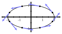
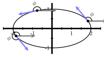
To measure the curvature, we first need to describe the direction of the curve at a point. We may do this using a continuously varying tangent vector to the curve, as shown at left in Figure 9.8.3. The direction of the curve is then determined by the angle \(\phi\) each tangent vector makes with a horizontal vector, as shown at right in Figure 9.8.3.
Figure 9.8.3 — Left: Tangent vectors to an ellipse. Right: Angles of tangent vectors.
Informally speaking, the curvature will be
the rate at which the angle \(\phi\) is changing as we move along the
curve. Of course, this rate of change will depend on how we move
along the curve; if we move with a greater speed along the curve,
then \(\phi\) will change more rapidly. This is why the speed limit is
sometimes lowered when we enter a curve on a highway. In other words,
the rate of change of \(\phi\) will depend on the parametrization we use
to describe the space curve. To eliminate this dependence on the
parametrization, we choose to work with an arc
length parametrization \(\vr(s)\), which means we move along the curve
with unit speed.
Using an arc length parametrization \(\vr(s)\), we define the tangent vector
\(\vT(s) = \vr'(s)\), and note that \(|\vT(s)| = 1\); that is, \(\vT(s)\) is
a unit tangent vector. We then have \(\vT(s) = \langle \cos (\phi(s)),
\sin(\phi(s)) \rangle\),
which means that
\[
\frac{d\vT}{ds} = \left\langle -\sin(\phi(s)) \frac{d\phi}{ds}, ~
\cos(\phi(s)) \frac{d\phi}{ds} \right\rangle =
\langle -\sin(\phi(s)),~
\cos(\phi(s)) \rangle \frac{d\phi}{ds}.
\]
This observation leads us to adopt the following definition.
Definition
If \(C\) is a smooth space curve and
\(s\) is an arc length parameter for \(C\), then the curvature, \(\kappa\), of \(C\) is
\[
\kappa = \kappa(s) = \left\lvert \frac{d \vT}{ds} \right\rvert.
\]
Note that \(\kappa\) is the Greek lowercase letter “kappa”.
Activity 9.8.5
We should expect that the curvature of a line is 0
everywhere. To show that our definition of curvature measures this
correctly in 2-space, recall that
(9.8.4) gives us the arc
length parameterization
\[
x(s) = x_0+\frac{a}{\sqrt{a^2+b^2}}s \ \ \ \ \text{ and } \ \ \ \
y(s) = y_0+\frac{b}{\sqrt{a^2+b^2}}s
\]
of a line. Use this information to explain why the curvature of a line is 0 everywhere.
Recall that an arc length
parameterization of a circle in 2-space of radius \(a\) centered at
the origin is, from
(9.8.3),
\[
\vr(s) = \left\langle a \cos\left(\frac{s}{a}\right),~
a \sin\left(\frac{s}{a}\right)\right\rangle.
\]
Show that the curvature
of this circle is the constant \(\frac{1}{a}\). What can you say about the relationship between the size of the radius of a circle and the value of its curvature? Why does this make sense?
The definition of curvature relies on our
ability to parameterize curves in terms of arc length. Since we have
seen that finding an arc length parametrization can be difficult, we
would like to be able to express the curvature in terms of a more
general parametrization \(\vr(t)\).
To begin, we need to describe the vector \(\vT\), which is
a vector tangent to the curve having unit length. Of course, the
velocity vector \(\vr'(t)\) is tangent to the curve; we simply need to
normalize its length to be one. This means that we may take
\[
\vT(t) = \frac{\vr'(t)}{|\vr'(t)|}.
\tag{9.8.5}\]
Then the curvature of the curve defined by \(\vr\) is
\[\begin{aligned}\kappa & = \left\lvert \frac{d \vT}{ds} \right\rvert \\
& = \left\lvert \frac{d \vT}{dt} \frac{dt}{ds} \right\rvert \\
& = \frac{\left\lvert \frac{d \vT}{dt} \right\rvert}{ \left\lvert \frac{ds}{dt} \right\rvert } \\
& = \frac{\text{|} \vT'(t) \text{|}}{ \text{|} \vr'(t) \text{|}}.\end{aligned}\]
This last formula allows us to use any parameterization of a curve to
calculate its curvature. There is another useful formula, given
below, whose derivation is left for the exercises.
Formulas for curvature
If \(\vr\) is a vector-valued function defining a
smooth space curve \(C\), and if \(\vr'(t)\) is not
zero and if \(\vr''(t)\) exists, then the curvature \(\kappa\) of \(C\)
satisfies
Use one of the two formulas for \(\kappa\) in terms of \(t\) to help you answer the following questions.
The ellipse \(\frac{x^2}{a^2} + \frac{y^2}{b^2} = 1\) has parameterization
\[
\vr(t) = \langle a\cos(t), b\sin(t) \rangle.
\]
Find the curvature of the ellipse. Assuming \(0 \lt b \lt a\), at what points is the curvature the greatest and at what points is the curvature the smallest? Does this agree with your intuition?
The standard helix has parameterization \(\vr(t) = \cos(t) \vi + \sin(t) \vj + t \vk\). Find the curvature of the helix. Does the result agree with your intuition?
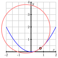
The curvature has another interpretation. Recall that the tangent line to a curve at a point is the line that best approximates the curve at that point. The curvature at a point on a curve describes the circle that best approximates the curve at that point. Remembering that a circle of radius \(a\) has curvature \(1/a\), then the
circle that best approximates the curve near a point on a curve whose curvature is \(\kappa\) has radius \(1/\kappa\) and will be tangent to the tangent line at that point and has its center on the concave side of the curve. This circle, called the osculating circle of the curve at the point, is shown in Figure 9.8.4 for a portion of a parabola.
Figure 9.8.4 — The osculating circle
Summary
The integration process shows that the length \(L\) of a smooth curve defined by \(\vr(t)\) on an interval \([a,b]\) is
\[
L = \int_a^b |\vr'(t)| \, dt.
\]
Arc length is useful as a parameter because when we parameterize with respect to arc length, we eliminate the role of speed in our calculation of curvature and the result is a measure that depends only on the geometry of the curve and not on the parameterization of the curve.
We define the curvature \(\kappa\) of a curve in 2- or 3-space to be the rate of change of the magnitude of the unit tangent vector with respect to arc length, or
\[
\kappa = \left\lvert \frac{d\vT}{ds} \right\rvert.
\]
Exercises
The WeBWorK problems are written by many different authors. Some authors use parentheses when writing vectors, e.g., \((x(t),y(t),z(t))\) instead of angle brackets \(\langle x(t),y(t),z(t) \rangle\). Please keep this in mind when working WeBWorK exercises.
1
Find the length of the curve
\[x = 3t-4,\quad y = 4t-4, z = 4-t,\]
for \(2 \le t \le 4\).
length = ___________________________________
(Think of second way that you could calculate this length, too,
and see that you get the same result.)
A factory has a machine which bends wire at a rate of 8 unit(s) of curvature per
second. How long does it take to bend a straight wire into a circle of radius
2?
_______________ seconds
\(0.0625\)
8
Find the unit tangent vector at the indicated point of the vector function
\[\mathbf{r}(t) = e^{4 t}\cos t \,\mathbf i +
e^{4 t}\sin t \,\mathbf j + e^{4 t} \,\mathbf k\]
Consider the moving particle whose position at time \(t\) in seconds is given by the vector-valued function \(\vr\) defined by \(\vr(t) = 5t \vi + 4\sin(3t) \vj + 4\cos(3t) \vk\). Use this function to answer each of the following questions.
Find the unit tangent vector, \(\vT(t)\), to the space curve traced by \(\vr(t)\) at time \(t\). Write one sentence that explains what \(\vT(t)\) tells us about the particle's motion.
Determine the speed of the particle moving along the space curve with the given parameterization.
Find the exact distance traveled by the particle on the time interval \([0,\pi/3]\).
Find the average velocity of the particle on the time interval \([0, \pi/3]\).
Determine the parameterization of the given curve with respect to arc length.
12
Let \(y = f(x)\) define a curve in the plane. We can consider this curve as a curve in three-space with \(z\)-coordinate 0.
Find a parameterization of the form \(\vr(t) = \langle x(t), y(t), z(t) \rangle\) of the curve \(y=f(x)\) in three-space.
Use the formula
\[
\kappa = \frac{\text{|} \vr'(t) \times \vr''(t) \text{|}}{\text{|} \vr'(t) \text{|}^3}
\]
to show that
\[
\kappa = \frac{\text{|} f''(x) \text{|}}{\left[1+(f'(x))^2\right]^{3/2}}.
\]
13
Consider the single variable function defined by \(y = 4x^2 - x^3.\)
Find a parameterization of the form \(\vr(t) = \langle x(t), y(t) \rangle\) that traces the curve \(y = 4x^2 - x^3\) on the interval from \(x = -3\) to \(x = 3\).
Write a definite integral which, if evaluated, gives the exact length of the given curve from \(x = -3\) to \(x = 3\). Why is the integral difficult to evaluate exactly?
Determine the curvature, \(\kappa(t)\), of the parameterized curve. (Exercise 12 might be useful here.)
Use appropriate technology to approximate the absolute maximum and minimum of \(\kappa(t)\) on the parameter interval for your parameterization. Compare your results with the graph of \(y = 4x^2 - x^3\). How do the absolute maximum and absolute minimum of \(\kappa(t)\) align with the original curve?
14
Consider the standard helix parameterized by \(\vr(t) = \cos(t) \vi + \sin(t) \vj + t \vk\).
Recall that the unit tangent vector, \(\vT(t)\), is the vector tangent to the curve at time \(t\) that points in the direction of motion and has length 1. Find \(\vT(t)\).
Explain why the fact that \(| \vT(t) | = 1\) implies that \(\vT\) and \(\vT'\) are orthogonal vectors for every value of \(t\). (Hint: note that \(\vT \cdot \vT = |\vT|^2 = 1,\) and compute \(\frac{d}{dt}[\vT \cdot \vT]\).)
For the given function \(\vr\) with unit tangent vector \(\vT(t)\) (from (a)), determine \(\vN(t) = \frac{1}{|\vT'(t)|} \vT'(t)\).
What geometric properties does \(\vN(t)\) have? That is, how long is this vector, and how is it situated in comparison to \(\vT(t)\)?
Let \(\vB(t) = \vT(t) \times \vN(t)\), and compute \(\vB(t)\) in terms of your results in (a) and (c).
What geometric properties does \(\vB(t)\) have? That is, how long is this vector, and how is it situated in comparison to \(\vT(t)\) and \(\vN(t)\)?
Sketch a plot of the given helix, and compute and sketch \(\vT(\pi/2)\), \(\vN(\pi/2)\), and \(\vB(\pi/2)\).
15
In this exercise we verify the curvature formula
\[
\kappa = \frac{\text{|} \vr'(t) \times \vr''(t) \text{|}}{\text{|} \vr'(t) \text{|}^3}.
\]
Use the fact that \(\vT(t) = \frac{\vr'(t)}{\text{|} \vr'(t) \text{|}}\) and \(\text{|} \vr'(t) \text{|} = \frac{ds}{dt}\) to explain why
\[
\vr'(t) = \frac{ds}{dt} \vT(t).
\]
In Exercise 14 we showed that \(\text{|} \vT(t) \text{|} = 1\) implies that \(\vT(t)\) is orthogonal to \(\vT'(t)\) for every value of \(t\). Explain what this tells us about \(\text{|} \vT(t) \times \vT'(t) \text{|}\) and conclude that
\[
\text{|} \vr'(t) \times \vr''(t) \text{|} = \left(\frac{ds}{dt}\right)^2 \text{|} \vT'(t) \text{|}.
\]
Finally, use the fact that \(\kappa = \frac{\text{|} \vT'(t) \text{|} }{\text{|} \vr'(t) \text{|}}\) to verify that
\[
\kappa = \frac{\text{|} \vr'(t) \times \vr''(t) \text{|}}{\text{|} \vr'(t) \text{|}^3}.
\]
16
In this exercise we explore how to find the osculating circle for a given curve. As an example, we will use the curve defined by \(f(x) = x^2\). Recall that this curve can be parameterized by \(x(t) = t\) and \(y(t)=t^2\).
Use (9.8.5) to find \(\vT(t)\) for our function \(f\).
To find the center of the osculating circle, we will want to find a vector that points from a point on the curve to the center of the circle. Such a vector will be orthogonal to the tangent vector at that point. Recall that \(\vT(s) = \langle \cos(\phi(s)), \sin(\phi(s)) \rangle\), where \(\phi\) is the angle the tangent vector to the curve makes with a horizontal vector. Use this fact to show that
\[ \vT \cdot \frac{dT}{ds} = 0.
\]
Explain why this tells us that \(\frac{dT}{ds}\) is orthogonal to \(\vT\). Let \(\vN\) be the unit vector in the direction of \(\frac{dT}{ds}\). The vector \(\vN\) is called the principal unit normal vector and points in the direction toward which the curve is turning. The vector \(\vN\) also points toward the center of the osculating circle.
Find \(\vT\) at the point \((1,1)\) on the graph of \(f\). Then find \(\vN\) at this same point. How do you know you have the correct direction for \(\vN\)?
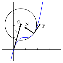
Let \(P\) be a point on the curve. Recall that \(\rho = \frac{1}{\kappa}\) at point \(P\) is the radius of the osculating circle at point \(P\). We call \(\rho\) the radius of curvature at point \(P\). Let \(C\) be the center of the osculating circle to the curve at point \(P\), and let \(O\) be the origin. Let \(\mathbf{\gamma}\) be the vector \(\overrightarrow{OC}\). See Figure 9.8.5 for an illustration using an arbitrary function \(f\).
Figure 9.8.5 — An osculating circle.
Which vector, in terms of \(\rho\) and \(\vN\) points from the point \(P\) to the point \(C\)? Use this vector to explain why
\[
\mathbf{\gamma} = \vr + \rho \vN,
\]
where \(\vr = \overrightarrow{OP}\).
Finally, use the previous work to find the center of the osculating circle for \(f\) at the point \((1,1)\). Draw pictures of the curve and the osculating circle to verify your work.