Section 12.3Using Parametrizations to Calculate Line Integrals
How can we use a parametrization of an oriented curve \(C\) to calculate \(\int_C\vF\cdot d\vr\)?
How does the parametrization chosen for an oriented curve \(C\) affect the value of the line integral \(\int_C\vF\cdot d\vr\)?
Under what conditions will changing the path taken from \(P\) to \(Q\) change the the value of the line integral?
We begin this section by taking a look at how to calculate a line integral of a vector field along different line segments. We will use this calculation as inspiration to see how treating oriented curves as vector-valued functions will allow us to quickly turn a line integral of a vector field into a single variable integral.
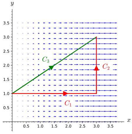
Let \(\vF=\langle xy,y^2\rangle\), let \(C_1\) be the line segment from \((1,1)\) to \((4,1)\), let \(C_2\) be the line segment from \((4,1)\) to \((4,3)\), and let \(C_3\) be the line segment from \((1,1)\) to \((4,3)\). Also let \(C = C_1 + C_2\). This vector field and the curves are shown in Figure 12.3.1.
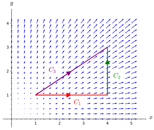
Every point along \(C_1\) has \(y=1\). Therefore, along \(C_1\), the vector field \(\vF\) can be viewed purely as a function of \(x\). In particular, along \(C_1\), we have \(\vF(x,1) = \langle x,1\rangle\). Since every point along \(C_2\) has the same \(x\)-value, write \(\vF\) as a function of \(y\) only (for the points on \(C_2\)).
\(\vF=\langle 4y,y^2\rangle \) along \(C_2\).
Recall that \(d\vr \approx \Delta \vr\), and along \(C_1\), we have that \(\Delta\vr = \Delta x\vi \approx dx\vi\). Thus, \(d\vr = \langle dx,0\rangle\). We know that along \(C_1\), \(\vF = \langle x,1\rangle\).
Use an analogous approach to write \(\int_{C_2} \vF\cdot d\vr\) as an integral of the form \(\int_c^d g(y)\, dy\) and evaluate the integral.
Along \(C_2\), \(d\vr = \langle 0,dy\rangle\) and \(1\leq y\leq 3\). Thus, we have \[ \int_{C_2} \vF\cdot d\vr = \int_1^3 y^2 dy = 9-\frac{1}{3} = \frac{26}{3}\].
Use the previous parts and a property of line integrals to calculate \(\int_C\vF\cdot d\vr\) without having to evaluate any additional integrals.
\[ \int_{C} \vF\cdot d\vr =\int_{C_1} \vF\cdot d\vr+\int_{C_2} \vF\cdot d\vr= \frac{15}{2}+\frac{26}{3}=\frac{97}{6} \]
Parametrizations in the Definition of \(\int_C\vF\cdot d\vr\)
In Preview Activity 12.3.1, you saw how line integrals along vertical and horizontal line segments can be done as integrals of a single variable. Before moving on to the general case, let us consider in the next example how we might tackle \(\int_{C_3}\vF\cdot d\vr\) in Figure 12.3.1.
Since \(C_3\) is from \((1,1)\) to \((4,3)\), we can determine that the line segment has slope \(2/3\), so we can write an equation for the line as \(y-1 = (2/3)(x-1)\) or \(y=\frac{2}{3}x+\frac{1}{3}\). Thus, along the curve \(C_3\), we can write \[ \vF=\left\langle \frac{2}{3}x^2+\frac{1}{3}x,(\frac{2}{3}x+\frac{1}{3})^2\right\rangle \]. Thinking of the slope of \(C_3\) as \(\Delta y/\Delta x\), we can write \(\Delta y/\Delta x = 2/3\), which can be rearranged to \(\Delta y = \frac{2}{3}\Delta x\). We may view \(\Delta\vr\) as \(\langle \Delta x,\Delta y\rangle\). Since \(\Delta x\approx dx\) and \(\Delta y\approx dy\), we use the fact that \(\Delta y = \frac{2}{3}\Delta x\) to write \(d\vr = \langle dx,\frac{2}{3}\, dx\rangle = \left\langle 1,\frac{2}{3}\right\rangle\, dx\). Along \(C_3\), we have \(1\leq x\leq 4\), so having rewritten \(\vF\) in terms of \(x\) and \(\vr\) in terms of \(dx\), we can now write \[\begin{aligned} \int_{C_3}\vF\cdot d\vr & = \int_1^4 \left\langle \frac{2}{3}x^2+\frac{1}{3}x,(\frac{2}{3}x+\frac{1}{3})^2\right\rangle \cdot \left\langle 1,\frac{2}{3}\right\rangle\, dx \\ & = \int_1^4 \frac{2}{3}x^2 + \frac{1}{3}x + \frac{2}{3}\left(\frac{2}{3}x + \frac{1}{3}\right)^2\, dx = \frac{151}{6} \end{aligned}\]. Notice that this result is different than what you obtained for \(\int_{C}\vF\cdot d\vr\) in Preview Activity 12.3.1, even though \(C\) and \(C_3\) both start at \((1,1)\) and end at \((4,3)\).
A recurring theme in this chapter will be the consideration of whether or not a vector field is a gradient vector field. Before moving on to generalize Example 12.3.1 to curves that are not line segments, it is worth examining this question for the vector field we have been investigating.
Is \(\vF=\langle xy,y^2\rangle\) a gradient vector field? Why or why not?
Preview Activity 12.3.1 and Example 12.3.1 have shown us that it is possible to evaluate line integrals without needing to work with Riemann sums directly. However, the approaches taken there seem rather cumbersome to use for oriented curves that are not line segments. It was not critical that the paths in Figure 12.3.1 were straight lines, but rather that the paths had a description where both \(x\) and \(y\) could be expressed in terms of one variable. Fortunately, parametrizing the oriented curve along which a line integral is calculated provides exactly the tool we are looking for. Namely a parameterization gives a way to express the points \((x,y,z)\) of the oriented curve in terms of a single variable (the parameter). Note that given a parameterization, we can also translate the vector field component equations into functions of the parameter as well.
In this example, we will look at the particulars of applying a parameterization of \(C\) (given by \(\vr(t) =\langle f(t),g(t)\rangle\) with \(t \in [a,b]\)) to . In particular, we will use this parameterization and a set of points along \(C\) that are equally spaced in terms of parameter values. To make this discussion a bit easier to read, we will work with a curve in two dimensions. However, all the ideas here generalize directly to curves in \(\R^3\).
Suppose that \(C\) is an oriented curve traced out by the vector-valued function \(\vr(t)\) for \(a\leq t\leq b\), and let \(\vF\) be a continuous vector field defined on a region containing \(C\). We can divide the interval \([a,b]\) into \(n\) sub-intervals, each of length \(\Delta t = (b-a)/n\), by letting \(t_i = a + i\Delta t\) for \(i = 0,1,\dots,n\). Dividing the interval \([a,b]\) into \(n\) pieces using \(t_i\) then can be used to break \(C\) up into \(n\) pieces by letting \(C_i\) be the part of the curve from \(\vr(t_{i})\) to \(\vr(t_{i-1})\) for \(i=1,\dots,n\).
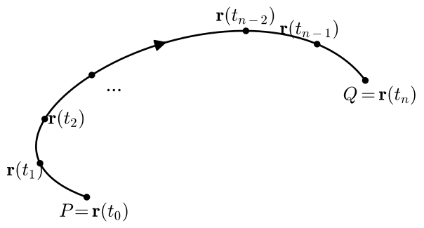
We can approximate the path \(C_i\) with the displacement vector \(\Delta \vr_i = \vr(t_{i}) - \vr(t_{i-1})\) as we did in Figure 12.2.6. Now notice that \[ \Delta \vr_i = \vr(t_{i}) - \vr(t_{i-1}) = \vr(t_{i} ) - \vr(t_{i} - \Delta t) = \left(\frac{\vr(t_{i} ) - \vr(t_{i}-\Delta t)}{\Delta t}\right) \Delta t \].
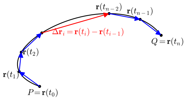
Our vector field for \(\int_C \vF \cdot d\vr\) can also be transformed into a function of \(t\) by substituting the \(x\) and \(y\) inputs with the corresponding components of the parameterization. If \(\vF= \langle F_1(x,y),F_2(x,y)\rangle\), then the parameterization given by \(\vr(t) =\langle f(t),g(t)\rangle\) means we can rewrite \(\vF\) as a function of \(t\): \[ \vF(t)=\vF(r(t))=\langle F_1(f(t),g(t)),F_2(f(t),g(t))\rangle \]
We can now substitute these pieces into Definition to obtain the following \[\begin{aligned} \int_C \vF\cdot d\vr & = \lim_{|\Delta \vr_i| \to 0} \sum_{i=1}^{n}\vF(\vr_i)\cdot\Delta\vr_i \\ & = \lim_{\Delta t \to 0} \sum_{i=1}^{n} \vF(\vr(t_i)) \cdot \left(\frac{\vr(t_{i}) - \vr(t_{i}-\Delta t)}{\Delta t}\right) \Delta t \end{aligned}\] When evaluating the limit as \(\Delta t\to 0\), the expression in the parentheses will be \(\vr'(t_i)\). We then have a Riemann sum that changes the evaluation of a line integral of a vector field along an oriented curve to a definite integral of a function of one variable. In particular, \[ \int_C \vF \cdot d\vr = \int\limits_a^b \vF(\vr(t))\cdot \vr'(t)\, dt \] Note that after evaluating the dot product, \(\vF(\vr(t))\cdot \vr'(t)\) is (scalar) function of \(t\).
We now state the general form of the preceding example as a theorem that will allow us to evaluate line integrals of vector fields in many contexts.
Let \(C\) be a smooth, oriented curve traced out by the vector-valued function \(\vr(t)\) for \(a\leq t\leq b\). If \(\vF\) is a continuous vector field defined near \(C\), then \[ \int\limits_C \vF\cdot d\vr = \int\limits_a^b \vF(\vr(t))\cdot \vr'(t)\, dt \].
To illustrate how useful Theorem is for evaluating line integrals, consider the following example.
Let \(\vF(x,y) = x\vi + y^2\vj\) and let \(C\) be the quarter of the circle of radius \(3\) from \((0,3)\) to \((3,0)\). This vector field and curve are shown in Figure 12.3.4. By properties of line integrals, we know that \(\int_C \vF\cdot d\vr = -\int_{-C}\vF\cdot d\vr\), and we will use this property since \(-C\) is the usual clockwise orientation of a circle, meaning we can parametrize \(-C\) by \(\vr(t) = \langle 3\cos(t),3\sin(t)\rangle\) for \(0\leq t\leq \pi/2\).
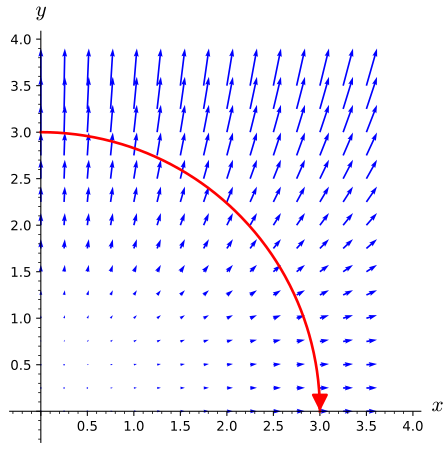
To evaluate \(\int_{-C}\vF\cdot d\vr\) using this parametrization, we need to note that \[ \vF(\vr(t)) = \langle 3\cos(t) , 9\sin^2(t)\rangle\qquad\text{ and } \qquad \vr'(t) = \langle -3\sin(t),3\cos(t)\rangle \]
Thus, we have \[\begin{aligned}\int_C\vF\cdot d\vr & = -\int_{-C}\vF\cdot d\vr \\ & = -\int_0^{\pi/2} \langle 3\cos(t),9\sin^2(t)\rangle\cdot\langle-3\sin(t),3\cos(t)\rangle\, dt \\ & = -\int_0^{\pi/2} \left(-9\sin(t)\cos(t) + 27\sin^2(t)\cos(t)\right)\, dt \\ & = -\int_0^1 (-9 u + 27u^2)\, du = -\left[ -\frac{9}{2}u^2 + 9u^3\right]_0^1 \\ & = -\left(-\frac{9}{2} + 9\right) = -\frac{9}{2}\end{aligned}\]. Note that we have used the substitution \(u =\sin(t)\) in evaluating the definite integral here.
As Example 12.3.3 shows, Theorem allows us to reduce the problem of calculating a line integral of a vector-valued function along an oriented curve to one of finding a suitable parametrization for the curve. Once we have such a parametrization, evaluating the line integral becomes evaluating a single-variable integral, which is something you have done many times before. The example also illustrates that using the properties of line integrals can allow us to use a more “natural” parametrization. You may find it interesting to use the parametrization \(\langle 3\sin(t),3\cos(t)\rangle\) for \(0\leq t\leq \pi/2\) to evaluate the line integral. Do you get the same result?
Find the work done by the vector field \(\vF(x,y,z) = 6x^2z\vi + 3y^2\vj + x\vk\) on a particle that moves from the point \((3,0,0)\) to the point \((3,0,6\pi)\) along the helix given by \(\vr(t) = \langle 3\cos(t),3\sin(t),t\rangle\).
\( \vr(t)=\langle 3\cos(t), 3\sin(t), t\rangle\) for \( 0\leq t\leq 6\pi\), so \( \frac{d\vr}{dt}(t) = \langle -3\sin(t), 3 \cos(t), 1 \rangle \), so \( \vF(t) =\langle 54t(\cos(t))^2, 27(s\sin(t))^2,3 \cos(t)\rangle \) and \[\int_C \vF \cdot d\vr =\int_0^{6\pi} -162t(\cos(t))^2\sin(t)+81(\sin(t))^2 \cos(t)+3\cos(t) \enspace dt=324 \pi\]
Let \(\vF(x,y) = \langle 0,x\rangle\). Let \(C\) be the closed curve consisting of the top half of the circle of radius \(2\) centered at the origin and the portion of the \(x\)-axis from \((2,0)\) to \((-2,0)\), oriented clockwise. Find the circulation of \(\vF\) around \(C\).
Let \(C_1\) be given by \( \vr(t) =\langle 2\cos(-t),2\sin(-t)\rangle\) where \(-\pi \leq t\leq 0\). This means that \(\vF(t) = \langle 0, 2\cos(-t) \rangle\) and \[ \int_{C_1} \vF\cdot d\vr =-4\int_{-\pi}^0 (\cos(t))^2 \enspace dt = -2 \pi\].
Let \(C_2\) be given by \( \vr(t) =\langle t,0\rangle\) where \(-2 \leq t\leq 2\). This means that \(\vF(t) = \langle 0, t \rangle\) and \[ \int_{C_2} \vF\cdot d\vr =\int_{-2}^2 0 \enspace dt = 0\].
Thus the line integral over \(C_1\) then \(C_2\) will give a result of \(-2\pi\).
Activity 12.3.4 will have you look at line integrals of the same vector field over several different types of curves. This will be an important, recurring theme as we study a variety of different integrals and vector fields in this chapter. In particular, we will use this approach of varying the region of integration for a fixed function several times in later activities.
Let \(\vF(x,y) = \langle y^2,2xy+3\rangle\).
Let \(C_1\) be the portion of the graph of \(y=2x^3+3x^2-12x-15\) from \((-2,5)\) to \((3,30)\). Calculate \(\int_{C_1}\vF\cdot d\vr\).
If \( \vF=\langle y^2,2xy+3\rangle \) and the curve \(C_1\) is traced out by \(\vr(t) = \langle t, 2t^3+3t^2-12t-15 \rangle \) for \(-2 \leq t\leq 3 \), then \[\int_{C_1} \vF\cdot d\vr =\int_{-2}^3 28t^{6} + 72t^{5} - 195t^{4} - 528 t^{3} + 180 t^{2} + 738 t + 189\, dt = 2825\]
Let \(C_2\) be the line segment from \((-2,5)\) to \((3,30)\). Calculate \(\int_{C_2}\vF\cdot d\vr\).
In this part, the curve \(C_2\) is traced out by \(\vr(t) =\langle -2+5t,5+25t \rangle\) for \(0 \leq t\leq 1\). So \[ \int_{C_2} \vF\cdot d\vr =\int_{0}^1 \langle (5+25t)^2,2(-2+5t)(5+25t)+3\rangle \cdot \langle 5,25\rangle \,dt = 2825\]
Let \(C_3\) be the circle of radius \(3\) centered at the origin, oriented counterclockwise. Calculate \(\oint_{C_3} \vF\cdot d\vr\).
In this part, the curve \(C_3\) is traced out by \(\vr(t) =\langle 3\cos(t),3\sin(t) \rangle\) as \(0 \leq t\leq 2\pi\). So \[ \int_{C_3} \vF\cdot d\vr =\int_{0}^{2\pi} \langle 9(\sin(t))^2,2\cos(t)\sin(t)+3 \rangle \cdot \langle -3\sin(t),3\cos(t) \rangle \, dt = 0\]
To connect the previous parts of this activity, use a graphing utility to plot the curves \(C_1\) and \(C_2\) on the same axes.
Alternative Notation for Line Integrals
In contexts where the fact that the quantity we are measuring via a line integral is best measured via a dot product (such as calculating work), the notation we have used thus far for line integrals is fairly common. However, sometimes the vector field is such that the units on \(x\), \(y\), and \(z\) are not distances. In this case, a dot product may not have quite the same physical meaning, and an alternative notation using differentials can be common. Specifically, if \(\vF(x,y,z) = F_1(x,y,z)\vi + F_2(x,y,z)\vj + F_3(x,y,z)\vk\), then \[ \int_C\vF\cdot d\vr = \int_C \langle F_1, F_2, F_3 \rangle \cdot \langle dx, dy, dz \rangle= \int_C F_1\, dx + F_2\, dy + F_3\, dz \]. A line integral in the form of \(\int_C F_1\, dx + F_2\, dy + F_3\, dz\) is called the differential form of a line integral. (If \(\vF\) is a vector field in \(\R^2\), the \(F_3\, dz\) term is omitted.) For example, if \(\vF(x,y,z) = \langle x^2y,z^3,x\cos(z)\rangle\) and \(C\) is some oriented curve in \(\R^3\), then \[ \int_C\vF\cdot d\vr = \int_C x^2y\, dx + z^3\, dy + x\cos(z)\,dz \]
It is important to recognize that the integral on the right-hand side is still a line integral and must be evaluated using techniques for evaluating line integrals. We cannot simply try to treat the line integral of the form \(\int_C F_1\, dx + F_2\, dy + F_3\, dz\) as if it were a definite integral of a function of one variable. Because the notation \(\int_C\vF\cdot d\vr\) provides a reminder that this is a line integral and not a definite integral of the types calculated earlier in your study of calculus, we will only use the vector notation for line integrals in the body of the text. However, some exercises may require the use of the differential form, and you may see the differential form used frequently in fields such as physics and engineering.
Independence of Parametrization for a Fixed Curve
Up to this point, we have chosen whatever parametrization of an oriented curve \(C\) was most convienent, and our argument for how we can use parametrizations to calculate line integrals did not depend on the specific choice of parametrization. However, it is not immediately obvious that different parametrizations don't result in different values of the line integral. Our next example explores this question.
Let \(\vF = x\vi\). We consider two different oriented curves from \((0,1)\) to \((3,3)\). The first oriented curve \(C\) travels horizontally to \((3,1)\) and then proceeds vertically to \((3,3)\). The second oriented curve \(C_3\) is the line segment from \((0,1)\) to \((3,3)\). Notice that, as depicted in Figure 12.3.5, we can break \(C\) up into two oriented curves \(C_1\) (the horizontal portion) and \(C_2\) (the vertical portion) so that \(C = C_1 + C_2\).
We first note that since \(\vF\) is orthogonal to \(C_2\), \(\int_{C_2}\vF\cdot d\vr=0\); therefore \(\int_C\vF\cdot d\vr =\int_{C_1}\vF\cdot d\vr\). We can parametrize \(C_1\) as \(t\vi+\vj\) for \(0\leq t\leq 3\) (\(t\) is treated like the coordinate \(x\)), which leads to \[ \int_{C_1}\vF\cdot d\vr = \int_0^3\langle t,0\rangle\cdot \langle 1,0\rangle\, dt = \int_0^3 t\, dt = \frac{9}{2} \].
Thus, \(\int_C\vF\cdot d\vr = 9/2\).
Now we look at \(\int_{C_3}\vF\cdot d\vr\), but we parametrize \(C_3\) in a nonstandard way by letting \(\vr(t) = \langle 3\sin(t),1+2\sin(t)\rangle\) for \(0\leq t\leq \frac{\pi}{2}\). (You should use a graphing utility to plot this parametrization to help convince yourself that it really does give \(C_3\).) This gives \(\vr'(t) = \langle 3\cos(t),2\cos(t)\rangle\), and \[\begin{aligned} \int_{C_3}\vF\cdot d\vr & = \int_0^{\pi/2}\langle 3\sin(t),0\rangle\cdot\langle 3\cos(t),2\cos(t)\rangle\, dt \\ & = \int_0^{\pi/2} 9\sin(t)\cos(t)\, dt = \frac{9}{2}\end{aligned}\].
In the next activity, you are asked to consider the more typical parametrization of \(C_3\) and verify that using it gives the same value for the line integral.
It's also worth observing here that \(\int_C\vF\cdot d\vr = \int_{C_3}\vF\cdot d\vr\), so at least two (very different) paths from \((0,1)\) to \((3,3)\) give the same value of the line integral here. The next section will further investigate when line integrals over different paths (with the same initial point and final point) will evaluate to the same value.
As promised, the final activity of this section (Activity 12.3.5) asks you to look at another parametrization of the curve \(C_3\) from the previous example. It also asks you to look at two different oriented curves between a pair of points, similarly to what you did in Activity 12.3.4.
The typical parametrization of the line segment from \((0,1)\) to \((3,3)\) (the oriented curve \(C_3\) in Example 12.3.4) is \(\vr(t) = \langle 3t,1+2t\rangle\) where \(0 \leq t\leq 1\). Use this parametrization to calculate \(\int_{C_3}\vF\cdot d\vr\) for the vector field \(\vF = x\vi\) and compare your answer to the result of Example 12.3.4.
Using the parametrization given the line integral becomes \[ \int_0^{1} \langle 3t,0\rangle \cdot \langle 3,2 \rangle \enspace dt = \int_0^1 9t \, dt = \frac{9}{2} \] This is the same result as in Example 12.3.4.
Calculate \(\int_C \langle (3xy+e^z), x^2, (4z+xe^z)\rangle\cdot d\vr\) where \(C\) is the oriented curve consisting of the line segment from the origin to \((1,1,1)\) followed by the line segment from \((1,1,1)\) to \((0,0,2)\).
Let \(\vr_1(t) = \langle t,t,t \rangle\) where\( 0 \leq t \leq 1\) and \(\vr_2(t) = \langle 1-t,1-t,1+t \rangle\) where\( 0 \leq t \leq 1\). Our line integral can be computed with \[ \int_{C_1} \vF \cdot d\vr = \int_0^1 \langle 3t^2+e^t,t^2,4t+te^t\rangle \cdot \langle 1,1,1\rangle \enspace dt= e+\frac{10}{3} \] \[ \int_{C_2} \vF \cdot d\vr = \\ \int_0^1 \langle 3(1-t)^2+e^{1-t},(1-t)^2,4(1+t)+(1-t)e^{1+t} \rangle \cdot \langle -1,-1,1\rangle \enspace dt \\ = 2e^2-3e+\frac{14}{3} \] Thus the line integral over \(C_1\) then \(C_2\) is \( 2e^2-2e+8\)
Calculate \(\int_{C'} \langle 3xy+e^z, x^2, 4z+xe^z\rangle\cdot d\vr\) where \(C_3\) is the line segment from \((0,0,0)\) to \((0,0,2)\).
The line segment from \((0,0,0)\) to \((0,0,2)\) can be given by \( \vr(t) = \langle 0,0,t \rangle\) with \( 0\leq t\leq 2\). Note that \(d\vr(t)= \langle 0,0,1 \rangle dt\), so \[\int_{C_3}\vF\cdot d\vr = \int_0^2 4t\enspace dt = 16\]
Is the vector field you considered in the previous two parts a gradient vector field? Why or why not? How does this compare to the vector field \(\vF\) of Activity 12.3.4?
No. One way to observe this would be to check the partial derivative with respect to \(y\) of the \(\vi\) component and compare it to the partial derivative with respect to \(x\) of the \(\vj\) component. Since they are not equal, Clairaut's Theorem tells us that this vector field is not a gradient vector field.
Although we have not given a proof or even an intuitive argument, the phenomenon you observed in part of Activity 12.3.5 is not particular to this curve or this vector field. The value of \(\int_C\vF\cdot d\vr\) does not depend on the parametrization of \(C\) used to calculate the line integral when using Theorem.
Summary
Line integrals of vector fields along oriented curves can be evaluated by parametrizing the curve in terms of \(t\) and then calculating the integral of \(\vF(\vr(t))\cdot \vr'(t)\) on the interval \([a,b]\).
The parametrization chosen for an oriented curve \(C\) when calculating the line integral \(\int_C\vF\cdot d\vr\) using the formula \(\int_a^b \vF(\vr(t))\cdot \vr'(t)\, dt\) does not impact the value of the line integral.
If \(C_1\) and \(C_2\) are different paths from \(P\) to \(Q\), it is possible for \(\int_{C_1}\vF\cdot d\vr\) to have a different value to \(\int_{C_2}\vF\cdot d\vr\).
Exercises
Suppose \(\vec{F}(x,y) = \langle e^x, e^y \rangle\) and \(C\) is the portion of the ellipse centered at the origin from the point \((0,1)\) to the point \((3,0)\) centered at the origin oriented clockwise.
(a) Find a vector parametric equation \(\vec{r}(t)\) for the portion of the ellipse described above for \(0 \leq t \leq \pi/2\).
\(\vec{r}(t) =\) ________________________________________
(b) Using your parametrization in part (a), set up an integral for calculating the circulation of \(\vec{F}\) around \(C\).
\(\displaystyle \int_C \vec{F} \cdot d \vec{r} = \int_a^b \vec{F}(\vec{r}(t)) \cdot \vec{r}'(t) \, dt = \int_a^b\) ________________________________________ \(dt\)
with limits of integration \(a =\) __________ and \(b =\) __________
(c) Find the circulation of \(\vec{F}\) around \(C\).
Circulation = ____________________
\(\left\langle 3\sin\mathopen{}\left(t\right),\cos\mathopen{}\left(t\right)\right\rangle\), \(3e^{3\sin\mathopen{}\left(t\right)}\cos\mathopen{}\left(t\right)-e^{\cos\mathopen{}\left(t\right)}\sin\mathopen{}\left(t\right)\), \(0\), \(\frac{\pi }{2}\), \(e^{3}-e^{1}\)
Evaluate the line integral \(\int_C \mathbf{F}\cdot d\mathbf{r}\), where \(\mathbf{F}(x,y,z) = -4x\mathbf{i} + 3y\mathbf{j} - 4z\mathbf{k}\) and C is given by the vector function \(\mathbf{r}(t) = \langle \sin t, \cos t, t \rangle, \quad \ 0\le t \le 3\pi/2.\)
____________________
\(-47.9132198049021\)
Evaluate the line integral \(\int_{\mathcal{C}} \mathbf{F} \cdot \,d\ \mathbf{r}\) where \(\mathbf{F}=\left\langle \sin x, \cos y, 10 xz \right\rangle\) and \(\mathcal{C}\) is the path given by \(\mathbf{r}(t) = (-2 t^3, -3 t^2, -3 t)\) for \(0 \le t \le 1\)
\(\int_{\mathcal{C}} \mathbf{F} \cdot \,d\ \mathbf{r}=\) ____________________
\(-34.725\)
Compute \(\int_{C_1} \vF\cdot d\vr\) when \(\vF=\langle x^2,xy\rangle \) and \(C_1\) is the line segment from \((0,0)\) to \((2,2)\).
The line segment \(C_1\) can be given by \( \vr(t) = \langle t,t\rangle\) as \( 0\leq t\leq 2\rangle\), which means that \(\vF \cdot d\vr=\langle t^2,t^2\rangle \cdot \langle 1,1\rangle \enspace dt=2t^2 dt\). Thus, \[ \int_{C_1} \vF \cdot d\vr=\int_0^2 2t^2 \enspace dt = \frac{16}{3}\]
Compute \(\int_{C_2} \vF\cdot d\vr\) when \(\vF=\langle x^2,xy\rangle \) and \(C_2\) is the line segment from \((2,2)\) to \((0,0)\).
This is the same integral as the previous part with the orientation flipped, so \[ \int_{C_2} \vF \cdot d\vr= -\int_{C_1} \vF \cdot d\vr= -\frac{16}{3}\]
If the wind in a region of space is given by \( \vF=\langle y+z,z-x,-z \rangle\) and a helicopter flies along the path given by \( \vr(t) = \langle 10 \sin(t),10\cos(t),(10-t)^2 \rangle\) as \(0\leq t\leq4\pi\). Calculate the work done by the wind on the helicopter.
Let \(C_3\) be the circle of radius \(7\) centered at the origin traveled counterclockwise. Compute \(\int_{C_3} \langle M, N\rangle\cdot d\vr\) when:
\(\langle M,N\rangle = \langle x,y \rangle\)
We will parametrize \(C_3\) by \(\vr(t) = \langle 7\cos(t),7\sin(t) \rangle\) as \(0\leq t\leq 2\pi \). So, \[ \int_{C_3} M\enspace x+N\enspace dy=\int_0^{2\pi} \langle 7\cos(t),7\sin(t)\rangle\cdot \langle-7\sin(t),7\cos(t)\rangle \enspace dt= 0 \]
\(\langle M,N\rangle = \langle -y,x \rangle\)
We will parametrize \(C_3\) by \(\vr(t) = \langle 7\cos(t),7\sin(t) \rangle\) as \(0\leq t\leq 2\pi \). So, \[ \int_{C_3} M\enspace x+N\enspace dy=\int_0^{2\pi} \langle -7\sin(t),7\cos(t)\rangle\cdot \langle-7\sin(t),7\cos(t)\rangle \enspace dt= 98\pi \].
\(\langle M,N\rangle = \langle 3,x \rangle\)
We will parametrize \(C_3\) by \(\vr(t) = \langle 7\cos(t),7\sin(t) \rangle\) as \(0\leq t\leq 2\pi \). So, \[ \int_{C_3} M\enspace x+N\enspace dy=\int_0^{2\pi} \langle3,7\cos(t)\rangle\cdot \langle-7\sin(t),7\cos(t)\rangle \enspace dt= 49\pi \].
Let \(C_4\) be the curve given by traveling along the path given by \( y=x^3-x\) on the surface given by \(z=xy\) as \(x\) goes from \(-1\) to \(2\). What is the work done by \(\langle x,z,x+y\rangle\)?